Topics (384k) Articles (398k) Users (410) Discussions (242) Comments (383) Files (13k) New article
Compare the qubit pure statewith , using the computational basis. Its Bloch vector is : it follows a meridian of the Bloch sphere from the north pole through to the south pole . The inner product with is , nonnegative on this interval. Consequently quantum fidelity, squared quantum fidelity, and trace distance areAt the triple is ; at it is ; at it is . The angle between the Bloch vectors is , while the quantum fidelity uses its half-angle. The pure-state trace distance and fidelity identity becomes the familiar relation .
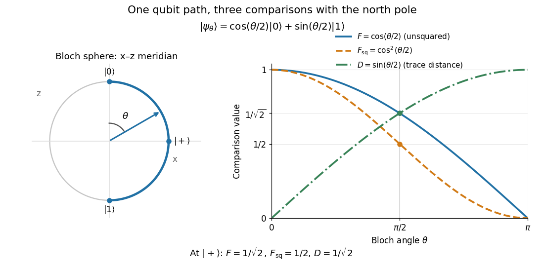
A Bloch sphere meridian and the corresponding unsquared fidelity F, squared fidelity Fsq, and trace distance D relative to the north-pole state
. Details. For equal prior probabilities, the Holevo–Helstrom theorem gives optimal quantum state discrimination success . Along this meridian it rises from to one, with at . This connects the geometric trace distance to the best possible decision from a single preparation; it is a different measurement task from the target-acceptance probability defining squared quantum fidelity.
// Target: quantum-information-theory.bigb
For the cubic polynomial, an oriented, normalized tangent vector isIts Euclidean norm is one and . The sign here follows increasing ; for a general solution branch, choose the sign of each new tangent vector so its dot product with the previous one is positive. First predict , then apply Newton method starting at toThe second equation keeps the correction on the transverse line in this two-dimensional example; in higher dimensions it is a hyperplane. Solving the linear system and updating corrects both coordinates together.
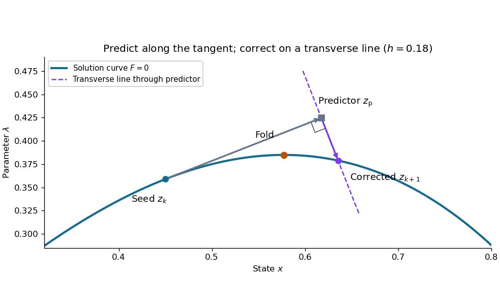
This step gives and . Check both equations: the solution must satisfy and . Checking only the first could accept any point on the solution branch. The new exceeds , so the step crosses the continuation fold, even though the predictor's exceeds .
At the seed, set . The determinant of the correction Jacobian matrix with the exact unit vector above isAt either continuation fold, , and : the correction remains invertible. More generally, if has full rank and a one-dimensional kernel spanned by , adding gives an invertible matrix, since a vector annihilated by both rows must be zero. This is a local argument; the old transverse hyperplane need not work arbitrarily far along the curve. Reduce and retry when correction fails, and check the equations and orientation after successful steps. Scaling state and parameter coordinates also matters, because it changes the Euclidean norm used to normalize the tangent vector.
// Target: analysis.bigb
For , choose independent random variables, each with the uniform distribution on a finite set , and decode their values as a Prüfer sequence. Every sequence has probability , and the bijection gives each labelled tree the same probability. This produces a uniform spanning tree of the complete graph without repeatedly proposing sets of edges and rejecting those that fail to be trees. It supplies random inputs for testing implementations of breadth-first search and a tractable model of random connections. [ref]
https://sites.math.rutgers.edu/~zeilberg/Combo20/hw.html. Doron Zeilberger, Rutgers Math 454 (2020), Lecture 23: generate random labelled trees by sampling and inverting Prüfer codes
This distribution is uniform over fixed-label trees, rather than over unlabelled trees. With four labels, the star graph shape has probability and the path graph shape has probability . Also, for a fixed label , the Prüfer degree formula givesHere the binomial distribution counts the independent code positions equal to . The expected value agrees with the average vertex degree from the degree-sum formula. Individual labels have the same distribution by symmetry, though their vertex degrees are constrained together by their fixed sum. When , simply return the single isolated vertex.
For a labelled tree with vertices, the vertex degree of label is one plus the number of occurrences of in its Prüfer sequence:Each recording of corresponds to an incident edge removed when a neighbouring leaf of a graph is deleted. Exactly one incident edge remains when itself is deleted, or when it belongs to the final pair. In particular, is a leaf of a graph exactly when it never occurs in the Prüfer sequence. The same reasoning applies to each remaining tree and its remaining code. [ref]
https://www.cs.columbia.edu/~cs4203/files/GT-Lec4.pdf. Columbia University, Graph Theory Lecture 4, Proposition 7.1: degree equals occurrences plus one
For , the occurrence counts in label order are , giving the degree sequence . Its sum is , as required by the degree-sum formula. More generally, summing the occurrence counts gives , so summing the vertex degrees gives .
In photoionization equilibrium at fixed gas density and temperature, the extra quasar photoionization rate reduces neutral-hydrogen column density by the displayed factor. Its local rate is calculated from the quasar flux, while the isotropic background rate is . Fitting the absorption suppression versus proper distance constrains the cosmic ionizing background. For an unperturbed column-density distribution proportional to with , the line abundance above a fixed threshold is reduced by . Density enhancement, quasar age, anisotropy and redshift errors must be distinguished from this ionization effect.
The displayed identity follows by testing the two possible truth values of . Existentially forgetting gives . Repeating this operation produces a propositional formula on a specified remaining vocabulary. Logical truth constants are needed if that vocabulary is empty.
In classical propositional logic, a truth value is false or true, encoded by a bit as zero or one. A Boolean valuation assigns these values to primitive propositions and extends to compound propositional formulas through logical connectives.
Write for aggregate route service. The four resource constraints are all sums of one odd and one even route service, so they are equivalent to the displayed maximum constraint. For fixed maxima, increasing each active service to its group's maximum improves weighted logarithmic utility. Maximizing with gives and , where , . Inactive routes are omitted; the same formula covers states where one group is empty.
Let the frailty random variable be uniform on with , and let the conditional individual hazard function be the constant , . Averaging conditional exponential survivor functions gives the displayed population survivor function for , with value one at zero. Its population hazard of a survival mixture isIt starts at and tends to : the frailty distribution among survivors progressively concentrates near its smallest frailty. Although each individual's hazard is constant, the population hazard decreases through survival selection.
Let a frailty random variable have a gamma distribution with mean one and variance . Its shape and rate are both . For conditional hazard function , , averaging the conditional survivor function gives . Differentiating its logarithm yields the population hazard function and hence the displayed hazard ratio. Writing gives . Therefore the population hazard ratio moves monotonically from towards one as exposure increases, even though the individual conditional hazard ratio remains . The limit one requires for fixed positive , or for fixed positive ; it is not a consequence of elapsed time alone. This is survival selection through preferential removal of larger frailties.
Every proper orthochronous Lorentz transformation is an exponential by  Codex 0 Created 2026-10-14 Updated 2026-10-25
Use the Lorentz spinor double cover . For a lift with distinct eigenvalues , diagonalize and choose logarithms ; this gives a traceless matrix logarithm. For a repeated eigenvalue, choose the sign of the lift so it is , where , and use . The two lifts have the same Lorentz image. Exponentiating the differential of the covering map therefore expresses every proper orthochronous transformation as the exponential of a real element of the Lie algebra of the Lorentz group. This argument does not assert that every element of itself has a traceless logarithm.
For affine complexified Minkowski space, the relevant twistor domain isIncidence can be written , absorbing the conventional factor into the definition of . Each space-time point gives a twistor line . On charts and , the fibre coordinates transform by , with , giving the two summands. The full projective twistor space corresponds to complexified compactified Minkowski space.
A linear transformation fixing every one-dimensional subspace is scalar. Fixing the coordinate lines makes it diagonal, and fixing the lines spanned by makes all diagonal entries equal. Within determinant-one matrices the scalar satisfies . Conversely scalars fix all projective points. Commutation with all elementary transvections shows these scalars are exactly the center of the special linear group, so its projective quotient acts faithfully.
A nonconstant morphism with would have a positive-dimensional fiber of a morphism by the fiber dimension theorem. A target hyperplane avoiding its image point meets the positive-dimensional projective image, so its pullback is a nonempty divisor in disjoint from that fibre. Every positive-dimensional projective subvariety meets every hypersurface: on its affine cone, a homogeneous equation cuts a positive-dimensional zero set containing a nonzero cone point. This contradiction proves constancy.
With the quotient convention, projective space represents the functor of surjections from a rank- free sheaf to a line bundle, modulo isomorphisms of the target compatible with the map. On an affine base the target may be a nontrivial rank-one projective module, so a tuple of elements generating the unit ideal is only the description when that target is trivial. Where the image of the th basis vector generates the target, divide the other images by it to get the usual affine coordinates. Infinitesimal variations of the quotient form and give the Euler sequence.
In an abelian category with enough projectives, a projective object has a resolution concentrated in degree zero, so every first left derived functor vanishes on it. Conversely choose with projective and use the additive functor with target the opposite of the category of abelian groups. This functor is right exact in that target. If , the derived exact sequence makes monic, meaning that is surjective in abelian groups. Extending gives a retraction of , so the sequence splits and is a direct summand of the projective .
For homogeneous fiber equations of fixed degrees in , put for . The linear map has image the degree- component of their homogeneous ideal. Hence it is surjective exactly when that ideal contains : the degree- monomials generate this power. In a family, the matrix entries are regular functions on the base. Failure of surjectivity is therefore a closed determinantal variety, cut out by the maximal-size matrix minors.
An invertible module over a commutative ring is a finitely generated module that is a projective module and whose localization at a prime ideal is free of rank one at every prime. Its dual module is also finite projective. Evaluation is an isomorphism after every prime localization, hence is an isomorphism globally by localization detects zero elements. The Picard group of a ring consists of the isomorphism classes of these modules under the tensor product of modules.
A finite projective module is a finitely generated module that is a projective module. Equivalently it is a direct summand of a finite free module: a finite free surjection splits by projectivity. Its dual module is finite projective and its evaluation map to its double dual module is an isomorphism, since both properties hold for finite free modules and pass to direct summands. Finite generation is needed for this elementary duality argument.
For a finite-dimensional algebra , a principal indecomposable module is an indecomposable direct summand of the left regular module, equivalently for a primitive idempotent . Its head of a module is simple, and it is the projective cover of that simple module.
Pinned article: Introduction to the OurBigBook Project
Welcome to the OurBigBook Project! Our goal is to create the perfect publishing platform for STEM subjects, and get university-level students to write the best free STEM tutorials ever.
Everyone is welcome to create an account and play with the site: ourbigbook.com/go/register. We belive that students themselves can write amazing tutorials, but teachers are welcome too. You can write about anything you want, it doesn't have to be STEM or even educational. Silly test content is very welcome and you won't be penalized in any way. Just keep it legal!
Intro to OurBigBook
. Source. We have two killer features:
- topics: topics group articles by different users with the same title, e.g. here is the topic for the "Fundamental Theorem of Calculus" ourbigbook.com/go/topic/fundamental-theorem-of-calculusArticles of different users are sorted by upvote within each article page. This feature is a bit like:
- a Wikipedia where each user can have their own version of each article
- a Q&A website like Stack Overflow, where multiple people can give their views on a given topic, and the best ones are sorted by upvote. Except you don't need to wait for someone to ask first, and any topic goes, no matter how narrow or broad
This feature makes it possible for readers to find better explanations of any topic created by other writers. And it allows writers to create an explanation in a place that readers might actually find it.
Figure 1. Screenshot of the "Derivative" topic page. View it live at: ourbigbook.com/go/topic/derivativeVideo 2. OurBigBook Web topics demo. Source. - local editing: you can store all your personal knowledge base content locally in a plaintext markup format that can be edited locally and published either:This way you can be sure that even if OurBigBook.com were to go down one day (which we have no plans to do as it is quite cheap to host!), your content will still be perfectly readable as a static site.
- to OurBigBook.com to get awesome multi-user features like topics and likes
- as HTML files to a static website, which you can host yourself for free on many external providers like GitHub Pages, and remain in full control

Figure 2. You can publish local OurBigBook lightweight markup files to either OurBigBook.com or as a static website.
Figure 3. Visual Studio Code extension installation.
Figure 5. . You can also edit articles on the Web editor without installing anything locally. Video 3. Edit locally and publish demo. Source. This shows editing OurBigBook Markup and publishing it using the Visual Studio Code extension. 
- Infinitely deep tables of contents:




All our software is open source and hosted at: github.com/ourbigbook/ourbigbook
Further documentation can be found at: docs.ourbigbook.com
Feel free to reach our to us for any help or suggestions: docs.ourbigbook.com/#contact