Topics (384k) Articles (398k) Users (410) Discussions (242) Comments (383) Files (13k) New article
A priority queue stores items with comparable priority keys and supports insertion, inspection of a best-priority item, and removal of a best-priority item. Here we use the minimum convention: keys have a total order, and smaller means earlier. The operation
peek returns a stored item of minimum priority without removing it; extract-min removes and returns such an item. Both require a nonempty priority queue, or an explicitly specified empty-case result. A maximum-oriented priority queue reverses the choice.For the requests ,
peek returns Bo and leaves all three requests stored. extract-min returns Bo and leaves Ada and Cy; another peek returns Cy. Inserting now makes Dee the next request selected. This changing collection need not be a sorted array: only the next choice must be available.Distinct items may share a priority. Inserting alongside permits either item to be removed first. A priority queue does not inherently promise arrival order on ties. If that policy matters, compare priority first and a unique increasing arrival number second; the resulting total order makes earlier arrivals win equal-priority ties. This is analogous to the motivation for stable sorting, but it is an extra policy for the priority queue.
The interface specifies behavior; the data structure determines costs. A binary heap implements a priority queue with constant-time
peek and logarithmic-time insertion and extract-min, under the cost assumptions below. Scheduling by urgency or by the time of the next event needs exactly this repeated next-item selection. MIT's notes use these applications to motivate the priority queue interface.[ref]https://ocw.mit.edu/courses/6-006-introduction-to-algorithms-spring-2020/40d4851e550507ca14dc778b9b2266cc_MIT6_006S20_lec8.pdf. MIT 6.006, lecture 8: priority queues and binary heaps, pp. 1–2
An adjacency list represents a graph by keeping, for each vertex , a collection of the vertices reached by its outgoing edges. An array indexed by vertex identifiers can locate each collection; the collection itself may use a linked list or an array. In an undirected graph, each nonloop edge supplies an entry at both endpoints.[ref]
Graph.java. Graph.java, class documentation and fields: vertex-indexed adjacency collections; addEdge: entries at both endpoints
For a worked example, take the simple graphwhere denotes the unordered pair . Its adjacency lists, displayed in label order, areThus has three neighbours, although the graph has six vertices. Its list contains exactly the destinations available for a single step from ; no slots are reserved there for . The fourteen neighbour entries represent seven edges, with appearing as in 's list and as in 's list. The label order makes the example easy to read; an adjacency list need not be sorted.
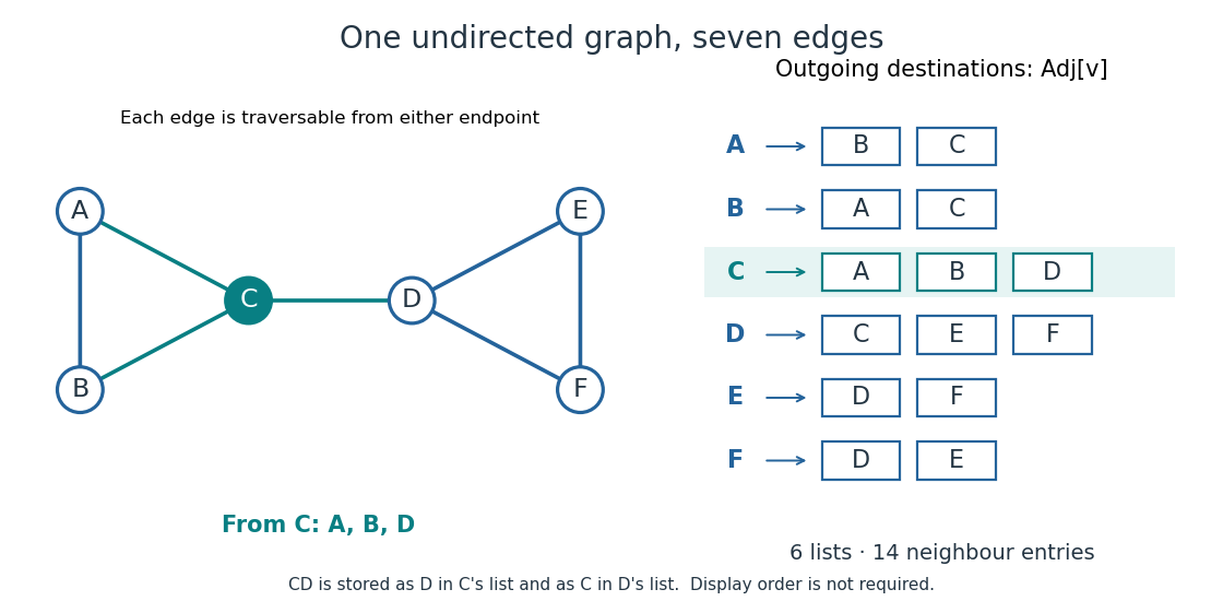
Seven undirected edges and their fourteen adjacency list entries
. Details. The useful idea is to store existing connections explicitly. Neighbour enumeration can then follow exactly the possible next steps, which is what breadth-first search and depth-first search need. In a sparse graph, most pairs of vertices have no edge; adjacency lists avoid reserving a separate adjacency matrix entry for every such absence. Whether this saves work depends on the question: neighbour enumeration and testing one proposed edge have different costs.
Image compression applies data compression to pictures, usually represented by raster images. Nearby pixels often have related shades; an encoder can exploit that structure. A flat region invites run-length encoding, while lossy block averaging trades fine detail for fewer stored samples. The choice depends on whether exact pixel values matter and on the patterns in the image.
Lossless source coding recovers the encoded pixel values exactly, including sharp text or numerical image data. Lossy compression preserves an approximation and can remove features that later image processing might need. A visually smooth result is therefore a different promise from exact recovery. Neither method has a universal compression ratio: the chosen file format, its file header and the particular image all matter.
PNG is a real format with lossless source coding of its encoded image data. Its specified compression uses Deflate on reversibly filtered rows, rather than our toy RLE format. The lossy block averaging example is also a teaching format, not a description of PNG. A lossy preprocessing step followed by saving as PNG preserves the already changed pixels, not the earlier original.[ref]
Portable Network Graphics (PNG) Specification (Third Edition) by Mark Adler and others. W3C, PNG Specification, Third Edition (2025), section 10, Compression
Deflate is the lossless source coding method specified for PNG compression. It can describe repeated stretches of earlier data, going beyond the single-value repetitions of run-length encoding.[ref]
Portable Network Graphics (PNG) Specification (Third Edition) by Mark Adler and others. W3C, PNG Specification, Third Edition, section 10.1, compression method 0
The format combines Deflate backreferences, which describe repeated stretches, with Deflate Huffman coding, which represents the resulting instructions using prefix codes. Deflate block framing tells the decoder which codes apply and where decoding stops. RFC 1951, DEFLATE Compressed Data Format Specification version 1.3 (May 1996), defines the format; different encoders can choose different instructions for the same input.[ref]
DEFLATE Compressed Data Format Specification version 1.3 by L. Peter Deutsch. RFC 1951, heading and sections 2 and 4: format and encoder choices
This separation is useful: discovering a repeated phrase and choosing short codewords solve different problems. A repeated phrase can contain many distinct bytes, while unequal codeword lengths can help even when no phrase repeats. Neither mechanism removes Deflate compression overhead or guarantees a saving on every input.
Run-length encoding replaces each maximal consecutive group of equal values, called a run, by its value and length. Decoding repeats each value the specified number of times. It is lossless source coding: no values are discarded. For a binary string, successive maximal runs alternate between 0 and 1, so storing the first bit and all run lengths is enough.
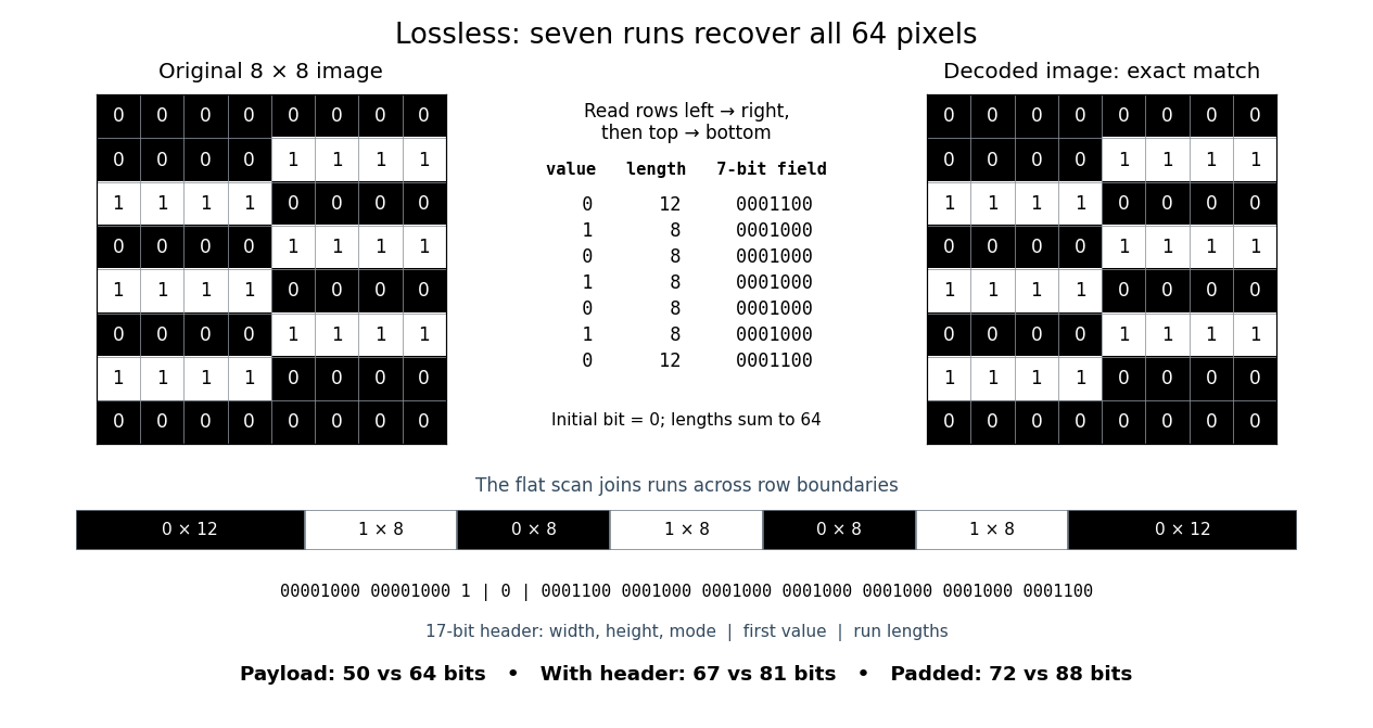
Take this raster image, with 0 black and 1 white, read left to right across each row and then top to bottom:Reading the whole image as one 64-bit binary string gives exactly seven runs:The lengths sum to . Repeating the alternating values for these lengths and splitting after every eighth pixel reconstructs every displayed row exactly.
00000000
00001111
11110000
00001111
11110000
00001111
11110000
00000000Here is a complete toy file format. Its file header is an eight-bit unsigned width, an eight-bit unsigned height, then a one-bit mode: 0 means raw pixels, 1 means run-length encoding. Fields are written most significant bit first; this profile accepts only width and height 8, so both decoders know to stop at 64 pixels. Raw mode contains 64 bits. RLE mode contains the initial bit, followed by seven-bit unsigned run lengths in the range 1 to 64. Zero and lengths above 64 are invalid; a decoder rejects a run that would exceed the remaining pixel count. It stops when the decoded lengths sum to 64, so no run-count field or end marker is needed.
For this image, the complete RLE serialization is:Spaces and vertical bars are explanatory separators, not stored characters. The seven-bit fields directly store the lengths; 64 would be
00001000 00001000 1 | 0 | 0001100 0001000 0001000 0001000 0001000 0001000 00011001000000. The payload costs bits, versus 64 raw bits. The 17-bit file header has the same size in either mode, giving complete sizes of 67 versus 81 bits. If packed into eight-bit units, append zero padding only at the end: the sizes become 72 versus 88 bits. These are sizes of this toy representation, not sizes of PNG files.The field design matters. Restarting RLE on every row costs eight initial bits plus four bits per run when lengths are stored directly: three bits represent only 0 through 7, whereas a row can have length 8. This pattern has row-run counts , totalling 14, so that payload costs bits, with no saving. Storing length minus one would instead fit lengths 1 through 8 into three bits, but is a different declared file format. An alternating flat 64-bit binary string has 64 runs and costs payload bits in our flat format; restarting each row costs payload bits. A one-run image costs only eight payload bits. These extremes explain when RLE is useful: long uninterrupted regions make short instructions, while frequent changes make instructions expensive.
Prefix codes of unequal lengths can replace fixed-width run lengths, provided the decoder knows the code and any necessary code description is counted. Run-length encoding names a technique, not one universal serialization. For a real implementation, Microsoft's bitmap documentation specifies
BI_RLE8 with count and value fields plus special commands, rather than our initial-bit convention.[ref]https://learn.microsoft.com/en-us/windows/win32/gdi/bitmap-compression. Microsoft, Bitmap Compression, BI_RLE8 encoded and absolute modes
Lossy compression reduces a representation while permitting irreversible changes to the original. The encoder can map distinct inputs to the same output, so its decoder cannot recover both originals exactly. The useful question becomes how much storage is saved for an acceptable amount of distortion: mean squared error is one numerical criterion, but it does not by itself measure how noticeable a visual change is.
For example, storing the arithmetic mean of four grayscale pixels retains their average shade while discarding their arrangement. Blocks and both produce 50. The former has detail and the latter is uniform, yet the decoder receives the same value. Lossy block averaging makes this ambiguity, its bit saving and its mean squared error exact.
Fix . There is no injective function from all length- binary strings to binary strings of length strictly less than . There are possible inputs, but even allowing the empty string gives onlypossible shorter outputs. The finite geometric series and pigeonhole principle leave at least two inputs sharing an output, which prevents exact decoding. For , eight inputs compete for the empty string and the six strings
0, 1, 00, 01, 10, 11.This counting argument includes any file header or other information sent to the decoder. An algorithm chosen separately for each input must also be identified to the receiver; its description is not free. A useful compressor saves space on some inputs while leaving others unchanged or making them longer. Lossy compression avoids the exact-recovery requirement by deliberately allowing several inputs to share an output.
Privacy amplification compresses a partially secret random string into a shorter key by a publicly selected hash function, reducing an adversary's information about the final key. In the BB84 protocol it follows parameter estimation and error correction, and accounts for information leaked in the public reconciliation transcript. Authentication of the public channel remains necessary.
A protocol for two distant parties to agree on a random bit without trusting either party to announce an unverified coin toss. In the Rabin-Williams scheme, a publicly committed square hides which of two half-interval roots the sender selected. The other party guesses a digit distinguishing those roots; subsequent root and factor revelations verify the completed exchange. The protocol's fairness relies on prescribed randomness and the difficulty of finding a second root; it does not force a party to complete communication.
Quantum key distribution uses a quantum channel and an authenticated public classical channel to establish matching random keys for two parties while limiting an eavesdropper's information. The public transcript is included in the adversary's information. In an ideal successful protocol, a key of length is uniform and independent of that information. Actual protocols allow small disagreement and secrecy errors and may abort. Measurement in quantum mechanics disturbance provides parameter tests, while privacy amplification removes residual knowledge after classical reconciliation. The BB84 protocol and entanglement-based protocols are examples.
A bit commitment allows a sender to fix a bit while concealing it from the receiver until an opening phase. Binding prevents a sender from opening the same commitment as either bit; hiding prevents the receiver from learning the bit prematurely. With a one-way permutation and a hard-core predicate , a commitment can consist of and the masked bit . Opening reveals . Injectivity gives binding, while unpredictability of the hard-core predicate gives computational hiding. For an RSA cryptosystem, the receiver must not possess the inverse trapdoor.
A hard-core predicate is an efficiently computable bit of an input to a one-way function that cannot be predicted from the function output with nonnegligible advantage over random guessing. For a one-way function , padding it to gives the inner-product predicate . This is the Goldreich–Levin construction. It provides a way to mask a bit using an otherwise publicly revealed one-way function value.
A one-way function is efficiently computable but computationally infeasible to invert on a randomly sampled input with nonnegligible success probability, under its stated security assumption. An RSA cryptosystem supplies the candidate map on units modulo . Inversion hardness is an assumption; it is not a proved consequence of merely choosing large primes.
On a finite rectangular Conway's Game of Life board stored as an array of Boolean variables, retain the preceding row's old values in one auxiliary row. Before overwriting a column, retain rolling sums of the old three-cell vertical columns. Their sum minus the old center is the old neighbor count. Read the next column before changing the current one; replace the saved row entry by the old current cell. The invariant is that every count uses the previous generation, just as in the two-array algorithm. For a board with rows and columns this uses auxiliary storage and time. The boundary convention must still be implemented explicitly. The Life blinker and Life glider provide exact expected generations for checking it.
The Life glider is a five-cell pattern that recreates its shape after four generations, shifted one cell along each coordinate. Use increasing rightward and increasing downward, as in the figure, and start from the live setEvery cell outside starts dead. Applying the Conway's Game of Life rule, rather than moving the drawing by hand, gives:
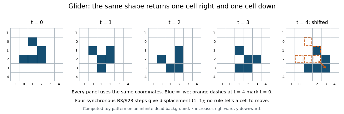
For an exact check of every frame, the intermediate live sets areHere means add to each ordered pair in . In the first step, the live cells and have respectively one and one live neighbors, so die; the other three have respectively three, three and two and survive. Exactly and are born, with three live neighbors each. This derives and explains how motion can occur while individual cells merely switch states.
Because the rule uses the same relative neighbors at every position, applying the global update function and applying a translation commute. Thus for every generation ; the four-step calculation establishes continued motion on the infinite board. The average displacement is cells per generation, or Euclidean distance per generation. The live-cell count happens to stay five in these frames, but the rule does not conserve live-cell count in general: a single isolated live cell dies immediately. The Life glider persists indefinitely in an otherwise empty infinite board; encounters with other patterns or a finite implementation's edge can change that conclusion.
// Destination: computer-science.bigb
A Life oscillator is a nonconstant periodic orbit of the Conway's Game of Life update function . Its period is the least positive integer for which , comparing the entire live-cell set at the same coordinates. A configuration that never changes is instead a fixed point; a Life glider is not a Life oscillator on the infinite board because it returns at displaced coordinates. The Life blinker has period two.[ref]
https://github.com/nathanieljohnston/game-of-life-book/blob/master/oscillators.tex. Johnston and Greene, chapter 3: oscillators and their periods
Publisher: Linux man-pages project.
This source is credited to an organization.
Online text: man7.org/linux/man-pages/man2/msync.2.html
Publisher: The kernel development community.
This source is credited to an organization.
Online text: docs.kernel.org/mm/page_cache.html
Cited passages: Page Cache, opening paragraph: normal reads, writes and mmaps go through the page cache; bypass paths exist.
The Open Group Base Specifications Issue 8, IEEE Std 1003.1-2024 by IEEE and others by  Codex 0 2026-10-13
By IEEE, The Open Group.
Publisher: IEEE and The Open Group.
This source is credited to an organization.
Pinned article: Introduction to the OurBigBook Project
Welcome to the OurBigBook Project! Our goal is to create the perfect publishing platform for STEM subjects, and get university-level students to write the best free STEM tutorials ever.
Everyone is welcome to create an account and play with the site: ourbigbook.com/go/register. We belive that students themselves can write amazing tutorials, but teachers are welcome too. You can write about anything you want, it doesn't have to be STEM or even educational. Silly test content is very welcome and you won't be penalized in any way. Just keep it legal!
Intro to OurBigBook
. Source. We have two killer features:
- topics: topics group articles by different users with the same title, e.g. here is the topic for the "Fundamental Theorem of Calculus" ourbigbook.com/go/topic/fundamental-theorem-of-calculusArticles of different users are sorted by upvote within each article page. This feature is a bit like:
- a Wikipedia where each user can have their own version of each article
- a Q&A website like Stack Overflow, where multiple people can give their views on a given topic, and the best ones are sorted by upvote. Except you don't need to wait for someone to ask first, and any topic goes, no matter how narrow or broad
This feature makes it possible for readers to find better explanations of any topic created by other writers. And it allows writers to create an explanation in a place that readers might actually find it.
Figure 1. Screenshot of the "Derivative" topic page. View it live at: ourbigbook.com/go/topic/derivativeVideo 2. OurBigBook Web topics demo. Source. - local editing: you can store all your personal knowledge base content locally in a plaintext markup format that can be edited locally and published either:This way you can be sure that even if OurBigBook.com were to go down one day (which we have no plans to do as it is quite cheap to host!), your content will still be perfectly readable as a static site.
- to OurBigBook.com to get awesome multi-user features like topics and likes
- as HTML files to a static website, which you can host yourself for free on many external providers like GitHub Pages, and remain in full control

Figure 2. You can publish local OurBigBook lightweight markup files to either OurBigBook.com or as a static website.
Figure 3. Visual Studio Code extension installation.
Figure 5. . You can also edit articles on the Web editor without installing anything locally. Video 3. Edit locally and publish demo. Source. This shows editing OurBigBook Markup and publishing it using the Visual Studio Code extension. 
- Infinitely deep tables of contents:




All our software is open source and hosted at: github.com/ourbigbook/ourbigbook
Further documentation can be found at: docs.ourbigbook.com
Feel free to reach our to us for any help or suggestions: docs.ourbigbook.com/#contact