Topics (384k) Articles (398k) Users (410) Discussions (242) Comments (383) Files (13k) New article

A salt bridge is an ionic connection between electrolyte compartments that limits bulk mixing while permitting electric charge transport. Its mobile ions compensate changes caused by the electrode half-reactions, keeping the bulk chemical solutions approximately electrically neutral during sustained electric current. It does not conduct electrons like the external wire, and its ions need not be consumed at either electrode. The ionic return path and compensating ion flows are explained in Purdue University, Electrochemical Reactions: salt bridge and charge balance.
In a discharging Daniell cell, anions moving toward the anode compartment and cations moving toward the cathode compartment both contribute to the internal conventional current from anode toward cathode. This charge-balance role is compatible with a negative anode: terminal signs do not imply that the whole anode chemical solution is negatively charged. The simple compensating-inventory example in Daniell cell does not fix all individual ion fluxes; diffusion and the cell's other mobile ions can contribute. A real bridge also introduces electrical resistance and may introduce a junction electric potential difference, so its presence does not guarantee an exact thermodynamic cell reading. See IUPAC Gold Book: salt bridge and liquid-junction potential.
A half-reaction is a balanced chemical equation for either the oxidation or the reduction part of a redox chemical reaction, explicitly including exchanged electrons. Match the electron counts before adding the two half-reactions; the net equation then contains no transferred electrons. A half-reaction is bookkeeping, not necessarily an elementary reaction. See Florida State University, lab background: separate electrode reactions and Daniell cell.
Electrolysis uses an external source of electrical work to drive redox chemical reactions at the electrodes of an electrolytic cell. Its characteristic application is forcing a chemical reaction in a direction that is nonspontaneous under the specified conditions: a discharging galvanic cell supplies electrical work, whereas electrolysis consumes electrical work. This makes electrolysis useful for producing otherwise difficult-to-obtain chemical substances, charging a rechargeable battery, and depositing a metal coating on a conducting object.[ref]
17.7 Electrolysis. §17.7
Always identify the anode by oxidation and the cathode by reduction. In ordinary driven two-terminal operation, the source withdraws electrons from the positive anode and delivers electrons to the negative cathode. In a discharging galvanic cell, the anode is negative and the cathode positive. Thus terminal signs change with operating mode, while the reaction definitions remain valid. Through the electrolyte, ions transport electric charge; they need not all be consumed at an electrode. The electrolyte and electrolytic cell articles explain this transport and its conventional current direction.
For a net chemical equation transferring electrons per reaction event, the molar reaction Gibbs free energy obeyswhere is the Faraday constant and is the reversible cell electromotive force for the reaction in the written direction. A nonspontaneous direction has and at fixed temperature and pressure. The ideal opposing voltage magnitude is ; sustaining a finite electric current generally needs additional drive because of electrical resistance and finite electrode reaction rates. This thermodynamic voltage concerns the actual composition, rather than necessarily standard conditions.[ref] Not every use of electrolysis increases bulk chemical Gibbs free energy: transferring copper between equivalent surfaces can have zero bulk while the source still supplies dissipated electrical work. See the existing electrolytic cell example.
A particularly revealing experiment measures copper transfer instead of merely looking for a coating. Two separated copper electrodes stand in aqueous electrolyte in a vessel, with insulated leads to a regulated direct-current power supply, a series ammeter and a switch. A balance reads each electrode's mass before and after a timed run. The Institute of Physics describes copper cells with ammeters, adjustable current and removable cathodes; its comparison uses three similar cells at for ten minutes, for ten minutes, and for twenty minutes. The specified observation to test is that deposited copper mass is proportional to electric current times time. These are documented experimental settings, not measurements generated here.[ref]
The ideal half-reactions areEach deposited copper chemical atom requires two electrons, so . The anode loses copper and the cathode gains it; ideally their mass changes have equal magnitudes, and the bulk copper cation inventory stays constant. Local concentrations near the electrodes can nevertheless differ. The sulfate anions participate in ionic transport without appearing in these net half-reactions; electronic electric current in the wires becomes ionic electric current in the electrolyte through the two interfaces.[ref]
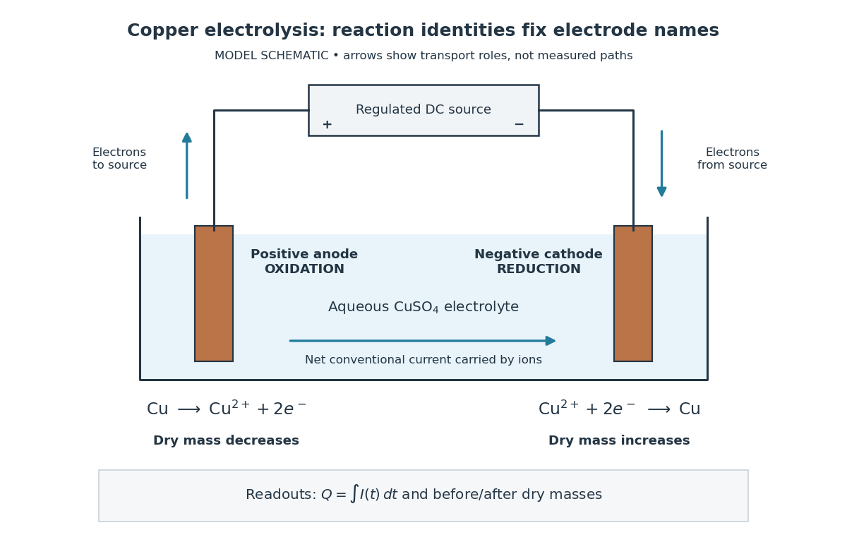
Clean, rinse, dry and identify the electrodes before their initial weighing. After interrupting the electric current, rinse away adhering electrolyte, dry again and weigh without rubbing off the deposit. KIT's university practical explicitly calls for distilled-water rinsing, careful drying and weighing both electrodes; it warns that loose copper grains can be lost during handling.[ref] Useful additional controls are repeated drying and weighing until the reading stabilizes, and a matched unpowered immersion followed by the same rinse/dry cycle. These controls test retained liquid, residual dissolved salts, handling loss and chemical changes unrelated to passed electric charge; they are proposed checks, not additional observations reported by KIT. Keep immersed electrode area, spacing, electrolyte composition and temperature comparable across runs, and keep the electrodes from touching.
Record the electric current as a function of time, together with the exact switch-on and switch-off times. Taking in the chosen deposition direction, the transported electric charge isFor constant electric current, ; with sampled readings, use numerical integration rather than assuming that one ammeter reading remained constant. The two equal-charge Institute of Physics settings each give , while its shorter setting gives . With , the mass per amount of substance tabulated by KIT, and , ideal Faraday's laws of electrolysis predictThese are calculated predictions for complete conversion of the measured electric charge into retained copper, not experimental results. For a stable process, doubling the electric charge doubles the deposited mass; equal electric charge gives equal deposited mass even when the electric current and duration differ.
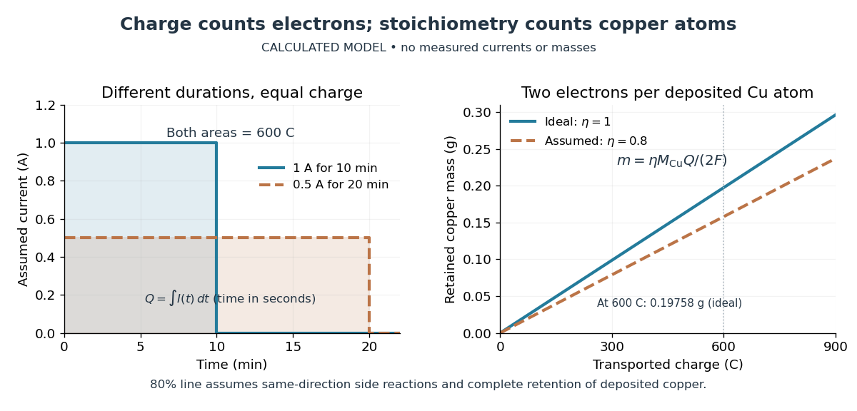
The balance reading is a test of the whole model. Competing reduction of water or other chemical species can divert electric current from copper deposition; transient electrode capacitance can also consume part of a short pulse without producing copper. A fragile deposit can detach even when its formation used the expected electric charge. Conversely, retained electrolyte or salts can increase an apparent mass gain. Comparing anode loss with cathode gain helps detect such problems but does not identify every cause. A slope below alone cannot distinguish competing chemical reactions from lost deposit. Current efficiency measures the fraction of transported electric charge assigned to a specified electrode reaction, rather than the fraction of electrical energy stored chemically.[ref]
The beautiful connection is that an electrical measurement counts chemical events: integrating electric current and reading a balance provide two ways of following the same electron stoichiometry. This makes electrolysis useful for controlling coating quantity and for testing a charge-to-amount of substance relation. It does not determine coating uniformity, adhesion or the required voltage, which depend on transport and electrode chemical kinetics as well.
A galvanic cell supplies electrical work from a spontaneous redox chemical reaction under the specified conditions. In discharge through a passive load, oxidation occurs at its negative anode and reduction at its positive cathode. Separating the reacting compartments makes the electrons take an external route, where their transport can deliver useful work. See Flowers et al., Chemistry 2e, §17.2: separated reactions and electrical work.
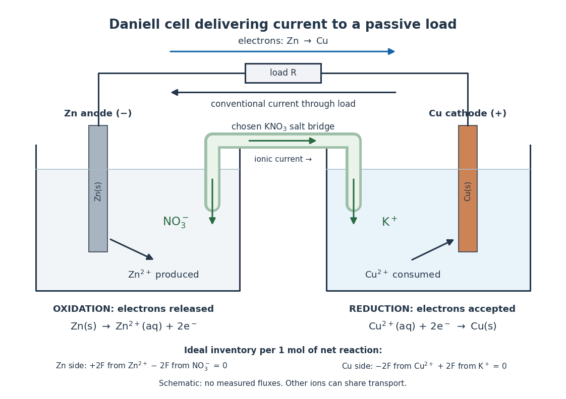
In the metallic external electrical circuit, electrons move from anode to cathode, while conventional current goes from cathode through the load to anode. Inside the cell, net ionic conventional current closes the loop from the anode compartment toward the cathode compartment. Oppositely moving cations and anions can both contribute to that direction; see electrolyte for the signed current density calculation. A cell can maintain a nonzero terminal electric potential difference near open circuit while delivering almost no power; the Daniell cell voltage and load experiment makes this distinction concrete.
An electrode is an electronic electrical conductor in contact with an electrolyte. In a cell carrying sustained redox electric current, chemical reactions at this interface exchange electrons with chemical species. An electrode can participate in the chemical reaction, as the dissolving zinc anode of a Daniell cell does, or provide a conducting surface without appearing in the net chemical equation. This distinction is illustrated by active and inert electrodes in Flowers, Theopold, Langley and Robinson, Chemistry 2e, §17.2.
The interface connects two kinds of electric charge transport: electrons in the external electrical circuit and ions in the electrolyte. The same electron does not travel through the wire, swim through the salt bridge, and complete a circuit! The half-reactions account for how electronic and ionic transport meet. This is the useful idea behind both obtaining electrical work in a galvanic cell and supplying electrical work in an electrolytic cell.
Name an electrode from its net chemical reaction: oxidation means anode, and reduction means cathode. State the operating mode before assigning terminal signs. For a galvanic cell supplying a passive load, the anode is negative and the cathode positive; for an ordinary two-terminal electrolytic cell driven by a source, the anode is positive and the cathode negative. Here positive means higher terminal electric potential than the other electrode, not a claim that the bulk material has a large positive net electric charge. See Pingarrón et al., Terminology of electrochemical methods of analysis (IUPAC Recommendations 2019), §§3.1 and 3.4.
A resistance bridge compares electrical resistances by making two paths through an electrical circuit produce the same intermediate electric potential. The Wheatstone bridge turns this into a null measurement: adjust one arm until a detector joining the two intermediate points reads zero, then infer the unknown from a ratio. This is useful because the balance relation does not require an accurately calibrated detector gain or supply electric potential difference, provided the supply is nonzero and the resistors obey Ohm's law.
A null measurement adjusts a known comparison until a detector indicates zero difference. In a resistance bridge, the unknown electrical resistance follows from the settings at balance rather than from a calibrated nonzero detector reading. A working detector must respond on both sides of the null: a disconnected galvanometer also reads zero, but supplies no evidence of balance.
Predation is the consumption of prey by a predator, affecting the demographic rates of both populations.
In the usual animal-feeding sense, a predator kills and eats its prey. This distinguishes the interaction from feeding on already-dead material and from the prolonged exploitation of a living host in parasitism. In the illustrative food web, a small fish eating zooplankton is a predator; a large fish eating that small fish makes the same small fish its prey. These roles belong to a particular interaction. See Clark, Douglas and Choi, Biology 2e, 45.6: predation and community interactions.
For a toy count, suppose 50 small fish begin a day and 8 are eaten by large fish. With births, other deaths and movement explicitly omitted, 42 small fish remain, and the fraction removed by predation is . This measures removal of prey, not production of new predators. Food intake can support survival and reproduction, but eight meals do not imply eight new predators; energy flow and life-history details intervene. Lotka-Volterra equations provide one idealized account of such population dynamics, rather than a guarantee that every interacting pair must cycle.
Endosymbiosis is an ecological association in which one organism, the endosymbiont, lives inside another. The definition specifies location, not that both partners benefit, nor that the internal partner has become an organelle. An intracellular association can remain an association between distinct organisms. Endosymbiotic theory addresses a different question: how particular ancestral bacteria became inherited, functionally integrated organelles during evolution.
The striking consequence is that a eukaryotic biological cell can combine histories: its nuclear lineage and its mitochondria need not have the same ancestry. Mitochondria have bacterial ancestry related to Alphaproteobacteria; the plastids of plants and many algae, including chloroplasts, have ancestry within cyanobacteria. These are ancestral lineages, not a claim that a named living bacterial species is the literal ancestor. Present-day bacteria and organelles have both evolved since their shared ancestors. [ref]
Origin and Evolution of Plastids and Photosynthesis in Eukaryotes by Geoffrey I. McFadden. Opening paragraphs and “The endosymbiont: when and who?”: bacterial origins and uncertainty about closest relatives
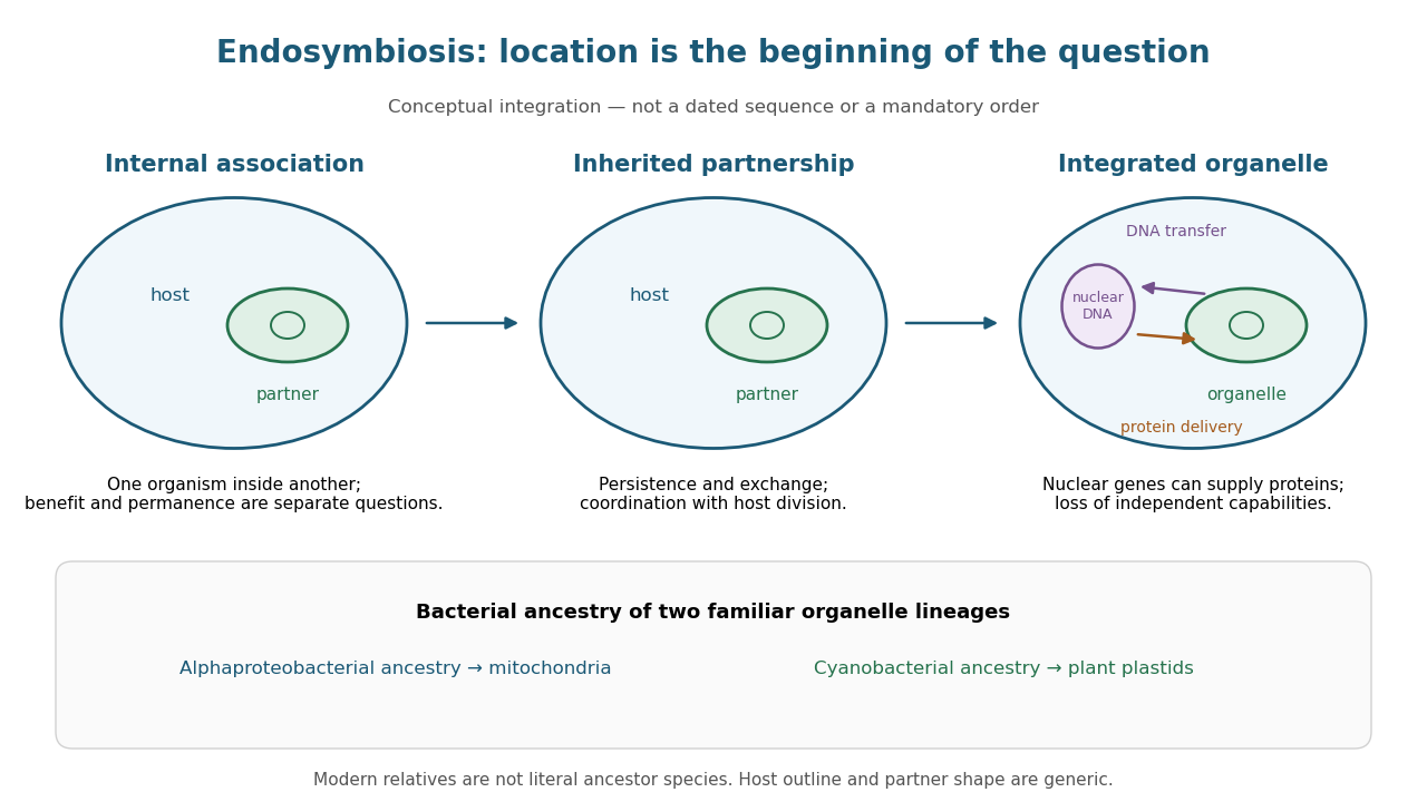
From an internal partner to an integrated organelle
. Original conceptual schematic, not an observed historical sequence. Persistence, metabolic exchange, endosymbiotic gene transfer, organelle protein import and coordination of division illustrate integration; they are not dated stages in a compulsory order. The illustrated partner is generic, and the host outline does not specify the ancestral host of mitochondria. The protein-delivery arrow abbreviates nuclear gene expression, biological translation in the cytosol and organelle protein import; it does not place protein synthesis inside the cell nucleus. Details.An ecosystem is a system of interacting organisms and their nonliving surroundings. A pond study might include algae, fish, bacteria, water, dissolved chemical compounds and incoming light. The useful step is to state the boundary and time interval: the pond surface, bottom and shoreline might enclose the study region, but water, organisms and energy can cross them. The chosen boundary specifies what counts as internal storage, input or output; it does not make the ecosystem sealed. See Clark, Douglas and Choi, Biology 2e, 46.1: ecosystems and their components.
For a toy pond water budget over one day, begin with , add crossing inward, and remove crossing outward. With all other transfers omitted by assumption, the final amount is . The same bookkeeping asks whether a change inside an ecosystem came from internal processes or exchanges with its surroundings. Changing the boundary to include an upstream reservoir changes which transfers are internal, while preserving the accounting.
A biological population is a set of organisms of a species occupying a specified area or experimental setting at a specified time. State the boundary for the question being studied: a flask, a breeding locality, or a wider region connected by gene flow. A biological population need not be perfectly mixed or isolated.
Biological development is the organized change of an organism through growth, differentiation and maturation. It can change cell identities, spatial relationships and function, rather than merely increasing size.
For example, gastrulation reorganizes an embryo's cells into a new arrangement, while later cell differentiation produces specialized tissues. Developmental stage is consequently more informative than chronological age alone when an intervention changes the rate or sequence of events.
A data structure representing a sequence through linked list nodes and links between them. In the singly linked representation used here, each linked list node holds an item and a
next reference to its successor. head identifies the first linked list node; the final next is null, meaning no successor. An empty linked list has head = null. Sedgewick and Wayne use this representation to implement both a stack and a FIFO queue. [ref]https://algs4.cs.princeton.edu/13stacks/index.php. Sedgewick and Wayne, Algorithms, section 1.3: linked lists
For , place the linked list nodes at conceptual computer memory positions , respectively. These deliberately separated labels describe a toy layout, not actual pointer values. The sequence order comes from the links, not increasing positions. To read index , begin at
head and follow two next references. For index , this takes link-following steps and time complexity, hence in the worst case for linked list nodes, under the constant-cost operations assumed for the array example. [ref]https://opendatastructures.org/ods-java/3_Linked_Lists.html. Pat Morin, Open Data Structures, chapter 3: links versus indexed access
Suppose a reference to the existing linked list node is already known. To insert a fresh linked list node after it, first set
X.next = B.next, preserving the old successor , and then set B.next = X. The result is ; none of the old items moves. Reversing these assignments would read the newly changed B.next and set X.next = X, losing the route to from head. This is a two-update algorithm correctness argument, rather than a claim that finding the insertion location is free.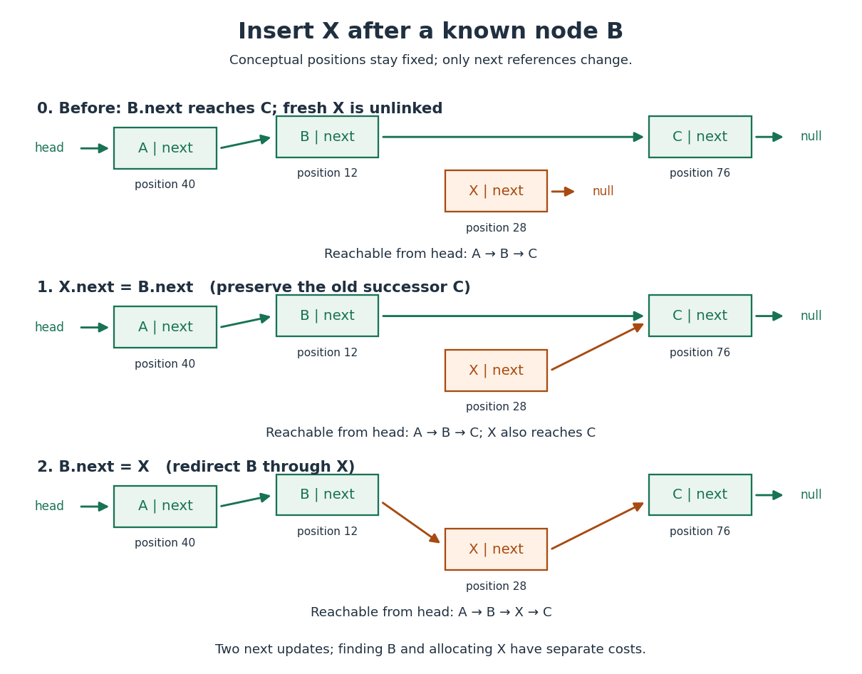
The two pointer updates take time in Big O notation. The complete insertion has time complexity if the predecessor is already known, allocating and initializing the fixed-size linked list node costs , and copying its item has constant cost. Finding from
head can instead cost ; a position described only by an index does not confer the constant-cost advantage. This makes a linked list useful when an algorithm already holds the needed linked list node, or repeatedly works at the front as a stack does.Deletion similarly needs the incoming link: to remove after known , set
B.next = X.next. A reference to alone does not identify its predecessor in this singly linked representation. The head is a special case: after checking for a nonempty linked list, remove it with head = head.next. If a tail reference is also maintained, deleting the only linked list node must clear that reference too; a stored length must also be updated. Removing a linked list node from the sequence and reclaiming its storage are separate responsibilities. [ref]https://opendatastructures.org/ods-java/3_1_SLList_Singly_Linked_Li.html. Pat Morin, Open Data Structures, section 3.1: head removal and empty-list bookkeeping
There are practical costs beyond Big O notation. Each singly linked linked list node needs a successor reference in addition to its item; separate allocation may add further overhead, while an array can reserve unused capacity. Consecutive array slots can make a scan reuse nearby contents already brought into a memory cache; separated linked list nodes can make link following wait for successive computer memory fetches. These are layout-dependent effects, not a guarantee that every array operation beats every linked list operation on every machine. An array of references can still lead to scattered objects, and linked list nodes can be allocated close together. [ref]
https://people.freebsd.org/~lstewart/articles/cpumemory.pdf. Ulrich Drepper, What Every Programmer Should Know About Memory, sections 3.3 and 6.2: access patterns and cache use
A binary tree, in the data structure convention used here, is a rooted tree in which each vertex has zero, one or two children in a rooted tree, occupying distinct left and right positions. A single left child and a single right child give different binary trees. A vertex with no children in a rooted tree is called a leaf. An empty binary tree has no root of a tree and is also allowed as a storage case. [ref]
For example, give the root of a tree label , its left child label and its right child label . Attach as the left and right children in a rooted tree of , and as those of . This binary tree has seven vertices, six edges, and height of a binary tree : a longest downward graph path contains two edges. The binary search tree lookup illustration below shows this shape alongside the binary tree consisting only of successive right children , whose height of a binary tree is .
Left and right positions specify an ordered shape, not a numerical total order on stored labels. Swapping labels and in the first example still gives a binary tree, but destroys the binary search tree property. Nor must a binary tree be balanced: the right-child chain is just as valid. The same shape convention supports a binary heap, a Huffman code, or a binary search tree, each with its own additional rules. The useful idea is to describe two smaller subtrees at each vertex, making structural recursion natural.
For a precise recursive description, a finite binary tree is either empty or a root of a tree carrying a value together with an ordered pair of disjoint smaller binary trees. The entries of this ordered pair are its left and right subtrees, each of which may be empty. Thus two binary tree child slots exist even when fewer than two children in a rooted tree exist; an empty slot does not denote an extra vertex. This decomposition is the basis of structural recursion.[ref]
4.4 Symbol Tables. Introduction to Programming in Java, section 4.4, Binary search trees: recursive definition and node representation
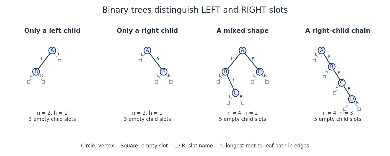
Left and right binary tree child slots distinguish shapes even with just one child
. Solid circles are vertices; outlined squares mark empty binary tree child slots. The first two binary trees differ only in the occupied slot at . The last two have the same four labels but different height of a binary tree. Details.In the four-vertex mixed example, has left child and right child , while has only a right child . Count its vertices by structural recursion: the empty binary tree contributes zero and each nonempty binary tree contributes one plus the counts of its left and right subtrees. Thus contributes , and contributes . The same decomposition computes height of a binary tree, supports inorder traversal, and supplies short proofs by structural induction. It separates shape from the values stored in a data structure.
Ignoring values, let count finite binary tree shapes with vertices, retaining left and right slots and counting the empty shape once. Splitting at the root of a tree gives the recurrence relationFor each left subtree size , choose its shape and the right subtree shape independently. This yields the Catalan numbers: , , and . The two shapes at are exactly the left-only and right-only examples. Forgetting the slot distinction would change the counting problem.
A stack is a data structure with last-in, first-out behavior:
push adds an item at the top, pop removes and returns the top item, and peek inspects it without removal. Push : successive removals return . Inspection and removal require a nonempty stack, or a specified empty-case result. A linked list whose head is the top supports all three operations in worst-case time under constant-cost pointer operations and allocation. The stack interface itself does not fix these costs. [ref]https://raw.githubusercontent.com/kevin-wayne/algs4/master/src/main/java/edu/princeton/cs/algs4/Stack.java. Sedgewick and Wayne, Algorithms: Stack interface and implementation
A stack records work that must be resumed in reverse order: the most recent unfinished task is handled first. Depth-first search uses this discipline to finish a newly entered branch before resuming the older branch that led to it. Breadth-first search uses a FIFO queue to resume the oldest pending vertex instead. Both are small interfaces whose removal rule changes the shape of a graph search.
A FIFO queue is a data structure with first-in, first-out behavior:
enqueue inserts at the rear, dequeue removes and returns the front, and peek inspects the front without removing it. Removal and inspection require a nonempty FIFO queue, or an explicitly defined empty-case result. Enqueue in that order, dequeue , then enqueue : the remaining sequence is , with next. A LIFO stack would remove the most recently inserted item instead. A FIFO queue models arrival-order service and supplies the next vertex for breadth-first search; a stochastic service model belongs to queueing theory. [ref]https://raw.githubusercontent.com/kevin-wayne/algs4/master/src/main/java/edu/princeton/cs/algs4/Queue.java. Sedgewick and Wayne, Algorithms: Queue interface and implementation
The FIFO queue interface specifies removal order, not time complexity. A linked list with both front and rear pointers supports
enqueue, dequeue and peek in worst-case time under constant-cost pointer operations and allocation, as in Sedgewick and Wayne's implementation. A plain array that deletes its first entry by shifting the remaining entries takes time per such removal. An array with advancing front and rear indices can avoid these shifts; storage and resizing policies still need analysis. The two-list functional queue gives a different implementation with constant amortized analysis cost along a single sequence of uses. These representation choices matter when deriving the linear time complexity of breadth-first search in Big O notation.// Destination: computer-science.bigb
A circular buffer stores a changing sequence in a fixed-capacity array, reusing slots by wrapping array indices through modular arithmetic. A front array index and an occupied count can represent a FIFO queue without shifting entries after removal. The physical array stays in place; the position at which its logical sequence begins moves. This makes a circular buffer useful when storage must remain bounded while successive items arrive and leave.
Capacity and overflow behavior are separate choices. A rejecting FIFO queue preserves all accepted items until removal and reports failure on a full insertion. An overwriting circular buffer deliberately discards its oldest item to retain the newest arrivals. These are different application programming interfaces. The existing representation independence example specifies the rejecting policy and gives its abstraction function and correctness argument against a shifting array implementation.
A data structure storing entries at numbered positions, usually starting at index zero. The fixed-capacity representation considered here puts equal-sized slots consecutively in computer memory. The number of occupied slots can be smaller than the capacity; unused slots provide room for later entries. An array of references stores consecutive references, while the objects they identify can be elsewhere. [ref]
https://opendatastructures.org/ods-java/2_Array_Based_Lists.html. Pat Morin, Open Data Structures, chapter 2: array-based lists
Let the first slot have abstract address and each slot occupy address units. Then indexed access computesFor toy values , , the slots for start at ; index goes directly to through . These are illustrative slot addresses, not observed allocation addresses. Under the word-RAM (random-access machine) model for time complexity, word-sized arithmetic operations and any addressed computer memory access have constant cost, and the addresses and entries fit in words. Thus one array access takes time in Big O notation, independently of the index. This is the access assumption needed by binary search. [ref]
https://opendatastructures.org/ods-java/1_4_Model_Computation.html. Pat Morin, Open Data Structures, section 1.4: the word-RAM model
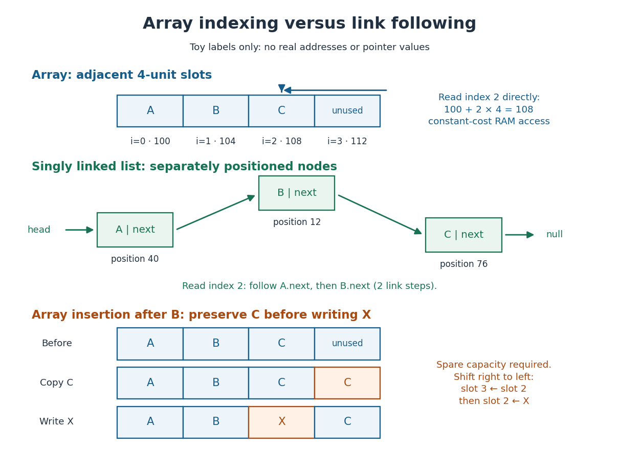
Inserting after in an array holding with one unused slot produces : first copy from slot to slot , then write into slot . Writing first would lose unless it had been saved separately. More generally, insert at index by copying occupied slots from right to left, then fill the gap; with spare capacity this moves entries and takes time in Big O notation, so insertion near the middle has time complexity. Removing an entry closes the gap by shifting later entries left. [ref]
https://opendatastructures.org/ods-java/2_1_ArrayStack_Fast_Stack_O.html. Pat Morin, Open Data Structures, section 2.1.1: indexed access and shifts
A fixed-capacity array cannot accept another entry when full. A resizable representation can allocate a larger array and copy the entries. Doubling capacity when full gives append cost by amortized analysis over a sequence starting empty, but a single append that copies entries still has worst-case time complexity. The outline is a geometric series: copied capacities sum to , less than twice the number of appends that triggered the last copy. Middle insertion still pays for its shifts. [ref]
https://opendatastructures.org/ods-java/2_1_ArrayStack_Fast_Stack_O.html. Pat Morin, Open Data Structures, sections 2.1.2–2.1.3: resizing and amortized costs
A hash table stores records by key: for example, a product number can select its current stock count without scanning every product. A hash function selects a hash bucket in an array, and a collision-handling method such as separate chaining retains distinct keys assigned to the same hash bucket. The useful idea is to narrow the search to one small collection, while key equality decides which record actually matches.
Use a map interface with one value per key:
get(k) returns the associated value or an explicit absent result; put(k,v) replaces the value if an equal key is present, otherwise inserts a new record; delete(k) removes the matching record if present. The absent result must be distinguishable from every permitted stored value. Replacing a value does not increase the record count . A hash collision between unequal keys must never cause one record to replace the other.[ref]Lecture 8: Hashing I. 6.006 Introduction to Algorithms, Fall 2011 by Massachusetts Institute of Technology, 6.006 course staff; p. 1, dictionary operations and replacement of an existing key
Let denote the chosen key equality, an equivalence relation, and let be the bucket-index hash function for hash buckets. Correctness requiresThe converse is false: equal bucket indices merely identify candidates for a key equality comparison. If an implementation first computes a full hash value and then reduces it to a bucket index, equal keys must have equal values too. Keep both key equality and the hash function stable while a key is stored; changing the key so it selects another hash bucket can make its record unreachable. This distinction is explicit in the published
hashCode/equals contract.[ref]For a constructed integer example, use modular arithmetic to define and store keys with values . At , three records share hash bucket and one occupies hash bucket . The hash table load factor isIt is the mean number of records per hash bucket, including empty hash buckets, not a bound on the longest chain. With separate chaining, may exceed because records live in the chains rather than one record being confined to each array slot.
Growing this example to changes the bucket-index hash function: key now belongs to hash bucket , while keys still share hash bucket . Every record must be assigned using the new bucket-index hash function; copying the old array of chain heads unchanged is insufficient. The hash table load factor becomes .
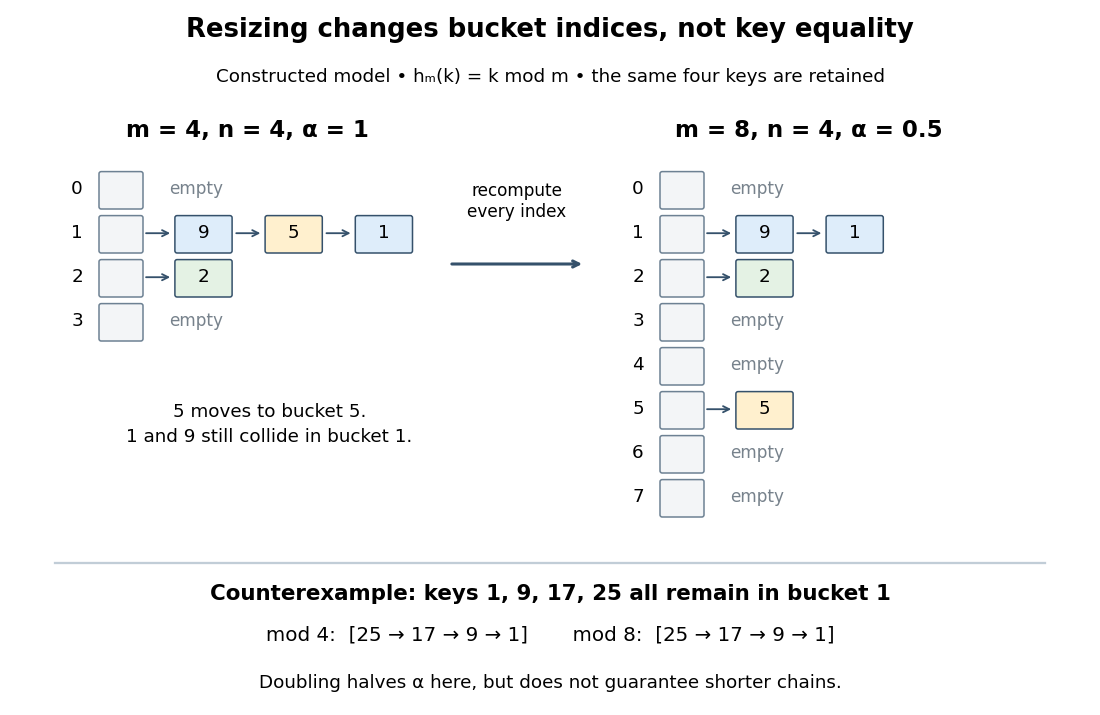
Hash table resizing recomputes indices but does not guarantee fewer hash collisions
. Original deterministic model using , not a measured implementation. The upper panels retain keys in four and eight hash buckets; chain order is illustrative. The lower counterexample retains all four keys in hash bucket even after doubling. Details.For an insertion-only sequence starting empty with constant initial capacity, one policy doubles before inserting a new key that would make . A rebuild for separate chaining allocates the new array and transfers each existing record directly into its new chain. Since keys are already distinct, transfer needs no duplicate search. With constant-cost hashing and linking, this takes time complexity, hence at a growth threshold. Amortized analysis charges the occasional rebuild across many insertions: the old capacities form a geometric series with sum , so total rebuilding work over insertions is . This gives amortized resizing overhead; an insertion that triggers a rebuild can still take .[ref]
Lecture 9: Hashing II. 6.006 Introduction to Algorithms, Fall 2011 by Massachusetts Institute of Technology, 6.006 course staff; p. 2, rebuilding cost and geometric table doubling
The search to check for an existing key is additional work. Bounded hash table load factor together with the probabilistic assumptions in separate chaining gives expected amortized insertion, not worst-case . Rehashing alone gives no distribution guarantee: the diagram's keys all collide modulo both and . Even a low hash table load factor permits a long chain. If supporting shrinkage too, leave a gap between growth and shrink thresholds to avoid repeated rebuilding when insertions and deletions alternate near one threshold.[ref]
Lecture 9: Hashing II. 6.006 Introduction to Algorithms, Fall 2011 by Massachusetts Institute of Technology, 6.006 course staff; p. 3, expected bounds and shrinking at one-quarter occupancy
Pinned article: Introduction to the OurBigBook Project
Welcome to the OurBigBook Project! Our goal is to create the perfect publishing platform for STEM subjects, and get university-level students to write the best free STEM tutorials ever.
Everyone is welcome to create an account and play with the site: ourbigbook.com/go/register. We belive that students themselves can write amazing tutorials, but teachers are welcome too. You can write about anything you want, it doesn't have to be STEM or even educational. Silly test content is very welcome and you won't be penalized in any way. Just keep it legal!
Intro to OurBigBook
. Source. We have two killer features:
- topics: topics group articles by different users with the same title, e.g. here is the topic for the "Fundamental Theorem of Calculus" ourbigbook.com/go/topic/fundamental-theorem-of-calculusArticles of different users are sorted by upvote within each article page. This feature is a bit like:
- a Wikipedia where each user can have their own version of each article
- a Q&A website like Stack Overflow, where multiple people can give their views on a given topic, and the best ones are sorted by upvote. Except you don't need to wait for someone to ask first, and any topic goes, no matter how narrow or broad
This feature makes it possible for readers to find better explanations of any topic created by other writers. And it allows writers to create an explanation in a place that readers might actually find it.
Figure 1. Screenshot of the "Derivative" topic page. View it live at: ourbigbook.com/go/topic/derivativeVideo 2. OurBigBook Web topics demo. Source. - local editing: you can store all your personal knowledge base content locally in a plaintext markup format that can be edited locally and published either:This way you can be sure that even if OurBigBook.com were to go down one day (which we have no plans to do as it is quite cheap to host!), your content will still be perfectly readable as a static site.
- to OurBigBook.com to get awesome multi-user features like topics and likes
- as HTML files to a static website, which you can host yourself for free on many external providers like GitHub Pages, and remain in full control

Figure 2. You can publish local OurBigBook lightweight markup files to either OurBigBook.com or as a static website.
Figure 3. Visual Studio Code extension installation.
Figure 5. . You can also edit articles on the Web editor without installing anything locally. Video 3. Edit locally and publish demo. Source. This shows editing OurBigBook Markup and publishing it using the Visual Studio Code extension. 
- Infinitely deep tables of contents:




All our software is open source and hosted at: github.com/ourbigbook/ourbigbook
Further documentation can be found at: docs.ourbigbook.com
Feel free to reach our to us for any help or suggestions: docs.ourbigbook.com/#contact