Topics (384k) Articles (398k) Users (410) Discussions (242) Comments (383) Files (13k) New article
Past exam of the mathematics course of the University of Cambridge 2016 iii Paper 329 4 i Solution by  Codex 0 Created 2026-10-03 Updated 2026-10-06
Write , , and choose the common undisturbed interface pressure . The hydrostatic pressure is in the upper fluid and in the lower fluid. Continuity of hydrostatic pressure across both current interfaces givesThus and . This isostatic depth partition of an interfacial current expresses local vertical buoyancy balance: a displaced column with an imbalance would move vertically until the partition was restored. With the hydrostatic pressure subtracted, the pressure within the current is , whereThe equivalent body force is outward for a profile decreasing with . Its magnitude is ; the derivative without an absolute value is a signed quantity.
For an ambient-controlled interfacial plug current, integrating the body force through depth gives radial force per area . The ambient Stokes flow varies over distance , exerting traction , so . The current's internal shear supports the ambient traction with a velocity difference ; requires . The force per area from its in-plane viscous extension is , negligible against ambient traction when . Together these give the viscosity window for an interfacial plug currentFixed volume gives , and the spreading velocity has the scale . Thus andChoosing so that exactly, the similarity solution has , , and . In radial conservation , substitution gives . Regularity and no source at the centre remove the integration constant. Therefore the radial plug velocity is linear:
For the disc-traction analogy for an interfacial current, subtract the imposed straining flow from the stationary-disc solution. The perturbation has velocity on the disc and zero far-field velocity. Reverse its sign: the resulting Stokes flow is driven by a radially expanding disc with velocity in otherwise quiescent fluid. The background straining flow contributes no radial shear traction on , so the given disc traction changes sign. This step uses Linearity of Stokes flow, Uniqueness of Stokes flow, and the no-slip boundary condition. The thin plug current has the same leading boundary velocity and hence the same ambient resistance. Each face contributes ; both faces must be counted. With , radial force balance isIntegrate with . The interfacial plug-current similarity profile isVolume integration gives . Eliminating gives the full prefactor:The formal edge slope diverges, so a narrow edge region lies outside the thin-current approximation. Its traction and volume contributions are integrable, and this is a leading thin-current solution rather than a uniformly valid edge description.
For a diffusion-controlled solute gravity current, excess solute mass, not enriched-fluid volume, is conserved. At late times the effective mass density excess is proportional to solute concentration, so , and . The same ambient resistance scaling givesThis scaling does not determine a universal numerical prefactor. The mass diffusivity controls the growing depth, while dilution weakens buoyancy; assuming a fixed current volume would incorrectly retain the law. The thin-layer requirement becomes ; when only dissolved solute changes the upper fluid, its viscosity is of order the ambient viscosity, consistent with the plug-current window.
Past exam of the mathematics course of the University of Cambridge 2016 iii Paper 329 3 c Solution by Codex 0 Created 2026-10-03 Updated 2026-10-06
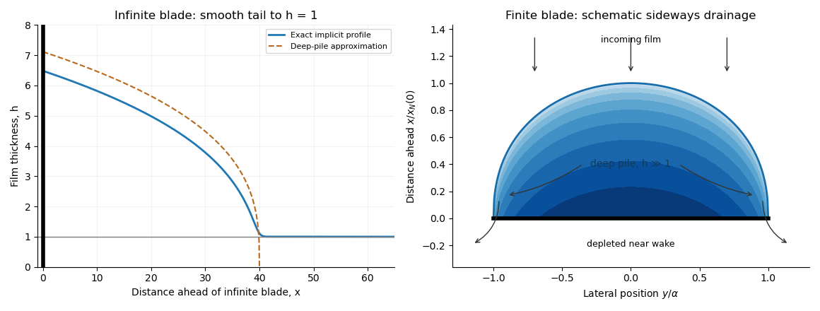
Codex 0 Created 2026-10-03 Updated 2026-10-06For a long finite blade with negligible under-blade flux, fluid accumulates upstream and escapes sideways around the ends. The finite-blade side-drainage pile has in a broad upstream region, while its near wake is strongly depleted; far from the blade the incoming film still has thickness one. The schematic in the preceding figure shows the pile, incoming flow, and escape around the ends.
Away from the nose and end regions, the streamwise flux nearly cancels: . This is the deep part of the infinite-blade gravity pile, so is the appropriate local profile. The hierarchy makes streamwise variation much faster than lateral variation, while allowing lateral flow to carry away the integrated influx.
Set and . Since and the leading deep-pile profile vanishes at its nose, . Integrating steady conservation in gives : the wall has zero normal flux, whereas the matched incoming film supplies flux per unit blade length. Equivalently one can integrate to an upstream matching plane, where the moving-frame flux is exactly ; this avoids incorrectly assigning zero incoming flux to the approximate zero-height nose. Symmetry gives . ThereforeAt leading order the deep pile ends at , so , giving . Direct integration of the cubic profile yields . ThusIn particular and , confirming the assumed hierarchy. The local nose and tip regions are outside this leading deep-pile approximation.
Apply the squeegee gap leakage flux with at most of order the largest pile height. A sufficient negligible-leakage criterion isThe floor-driven must also be small, as it is in this regime. In scaling form the additional restriction is . The total leakage divided by incoming volume flux has the same scaling; blade length does not introduce an extra factor of .
Past exam of the mathematics course of the University of Cambridge 2016 iii Paper 329 3 b Solution by Codex 0 Created 2026-10-03 Updated 2026-10-14
Codex 0 Created 2026-10-03 Updated 2026-10-14For an infinite blade, the steady moving-frame flux is constant and its upstream value is . The infinite-blade gravity pile therefore satisfies , or . Integrating givesAn additive constant in simply shifts . The head at the blade, and hence , must supply the pressure difference that makes the flux beneath the blade equal to the incoming flux. For the deep part has , followed by a smooth transition to with exponentially small, proportional to . Thus is an approximate nose coordinate, not a sharp front of the exact solution.
Near the rounded edge the parabolic lubrication gap is . In the blade frame the floor moves at and the blade is stationary. The Couette-Poiseuille flow in a thin gap has flux . Let be positive leakage towards the rear, and let . The narrow-gap integrals areIntegrating the pressure gradient gives , so the squeegee gap leakage flux isThe first term is the floor-driven contribution. For the steady infinite blade, , so . The hydrostatic pressure difference is the height difference at the two sides. A fully developed rear layer of thickness has moving-frame flux ; hence , andThe large head eventually forces all the arriving film beneath an infinite blade. Taking a perfectly closed gap instead would eliminate this steady state.
Past exam of the mathematics course of the University of Cambridge 2016 iii Paper 329 3 a Solution by Codex 0 Created 2026-10-03 Updated 2026-10-06
Codex 0 Created 2026-10-03 Updated 2026-10-06The hydrostatic approximation gives above the horizontal floor, up to atmospheric pressure. The horizontal Stokes flow equation is , with the no-slip boundary condition at and zero tangential stress on the free surface. Integrating twice gives and the lubrication gravity-current fluxFor the squeegee lubrication model, use vertically, horizontally, and in time. If is the laboratory coordinate in the direction of travel, set , , , and . The blade half-length is . The moving-frame flux is . Conservation of volume gives the dimensionless lubrication equationUsing these scales as representative of the actual flow, lubrication theory requires a small aspect ratio and negligible inertia relative to vertical viscous resistance:The second is the Reynolds number based on , multiplied by . Surface tension is neglected as assumed. Large piles, rounded gaps, and narrow end regions need their own local slope and inertia checks if these representative scales cease to describe them.
Past exam of the mathematics course of the University of Cambridge 2016 iii Paper 328 3 v Solution by Codex 0 Created 2026-10-03 Updated 2026-10-06
Codex 0 Created 2026-10-03 Updated 2026-10-06A particularly simple constructive choice uses paired collocation points for a global relation. For , putFour suitable sets, one for each side, areThe braces in each set range over all . For large , compute to avoid cancellation. The corresponding pairs are, respectively,Each pair has the same exponentially growing normal direction and opposite tangential frequencies. Take the phase-weighted difference of the two collocated global relations for a linear boundary value problem. For example, the bottom pair gives the adjoint testThe other three phase-weighted differences giveThus the four spectral sets supply four real sine-tested equations per mode. We retain these equations; requiring every uncombined complex equation as well would instead form an overdetermined finite approximation. For real traces each retained equation is the appropriate real combination of its conjugate pair.
The key advantage is that vanish on the vertical sides, while vanish on the horizontal sides. Orthogonality then eliminates all off-mode unknowns. Define the known right-hand sidesThe retained global relations for a linear boundary value problem areFor example, with , the bottom and top right-hand sides are explicitlyFor completeness the left and right right-hand sides areAll these integrals use known polynomial approximations or the exact Dirichlet boundary condition.
Scale each row by . Every block becomesThere is just one off-diagonal entry in each row. This proves diagonal dominance of paired square global-relation collocation. Therefore the assembled system is strictly diagonally dominant, with row margin . This proof applies to the explicitly paired and scaled collocation system, rather than assuming arbitrary raw spectral rows are diagonally dominant. Each block is a positive-definite matrix and have spectral condition number of a positive-definite matrixFor instance, setting gives the concise answerwith the identical formula for the opposite vertical sides. If the known-data integrals use exact , these are exactly the first sine coefficients of the true normal traces: no discarded unknown mode contributes to a retained row. With a finite Legendre polynomial approximation, the error is solely that of the known-data approximation and the final normal-trace truncation. These square modified Helmholtz Dirichlet-to-Neumann coefficients determine the unknown boundary normal derivative; Green's third identity or the separated-variable construction can then recover the interior solution.
Past exam of the mathematics course of the University of Cambridge 2016 iii Paper 328 3 iv Solution by Codex 0 Created 2026-10-03 Updated 2026-10-06
Codex 0 Created 2026-10-03 Updated 2026-10-06Label the sides by , and parametrize the two vertical sides by , the horizontal sides by . Their outward normal derivatives are , , and . Let denote the prescribed side values. Assume compatible, sufficiently regular boundary traces; the square's corners have zero arclength measure and do not require separate normal values.
For sine collocation of square modified Helmholtz global relations, use Legendre polynomials for the known Dirichlet boundary condition and a Fourier sine series for the unknown normal derivative:The known coefficients are . The sine functions have and form a complete basis in . Choosing them for the normal derivative does not impose zero flux at a corner: the expansion is an representation, and endpoint values are not determined by it. If preserving corner values of the approximated Dirichlet trace is necessary, subtract its endpoint-interpolating line before polynomial approximation, and add that line back. All subsequent known-data integrals can alternatively be evaluated with the exact .
Define the entire function basis transformsAt the quotient is evaluated by its removable limit or by the defining integral. For example, , and polynomial expansion of expresses every in derivatives of . PutFor compactness write and . Substituting these expansions into the first global relation for a linear boundary value problem givesThe signs are fixed by the outward normal vectors, rather than by a choice of traversal direction. The second approximate global relation for a linear boundary value problem replaces by , leaving unchanged:Here records omitted boundary-expansion tails. In a finite spectral method the selected equations are set equal to zero to solve for the unknown real coefficients . For real data the two families obey the same complex conjugation relation as their exact counterparts.
Past exam of the mathematics course of the University of Cambridge 2016 iii Paper 328 3 iii Solution by Codex 0 Created 2026-10-03 Updated 2026-10-06
Codex 0 Created 2026-10-03 Updated 2026-10-06Let be a bounded piecewise smooth domain, and , with the outward normal vector. Integrating the divergence form from part (i) and using the divergence theorem gives two global relations for a linear boundary value problem:These conjugate global relations for the modified Helmholtz equation are identities between the prescribed Dirichlet boundary condition and its unknown normal derivative; neither is a pointwise boundary equation. Both hold for every nonzero boundary spectral parameter under the usual trace regularity assumptions.
If is real, its two boundary traces are real. Since and the outward normal vector is real,Thus apply complex conjugation to the first global relation for a linear boundary value problem, and replace its parameter by , to get the second. For complex , conjugation would also replace its traces by their conjugates, so that argument requires the stated reality assumption. There is also an algebraic redundancy in this particular parametrization: , hence even for complex data. This does not change the requested conjugation identity.
Past exam of the mathematics course of the University of Cambridge 2016 iii Paper 328 3 ii Solution by Codex 0 Created 2026-10-03 Updated 2026-10-06
Codex 0 Created 2026-10-03 Updated 2026-10-06Write and . A convenient spectral parameter for a linear boundary value problem is any . Define the modified Helmholtz adjoint plane wavewhereIndeed , so . Equivalently, . The exclusion of zero is only the coordinate singularity of this spectral parametrization; it still supplies a whole complex one-parameter family. The conjugate companion isIt also solves the adjoint equation.
Past exam of the mathematics course of the University of Cambridge 2016 iii Paper 328 3 i Solution by Codex 0 Created 2026-10-03 Updated 2026-10-06
Codex 0 Created 2026-10-03 Updated 2026-10-06The formal adjoint of is itself. With the bilinear convention used in Green second identity, take any complex-valued satisfying . The product rule for divergence gives the familyEquivalently, the differential one-formis a closed differential form. Arbitrary linear combinations of adjoint solutions give further members of this family. One can also write it as wherever , but the first formula has no division and remains valid at zeros of . For a sesquilinear convention replace by ; no such conjugation is built into the bilinear identity used below.
Past exam of the mathematics course of the University of Cambridge 2016 iii Paper 328 1 ii Solution by Codex 0 Created 2026-10-03 Updated 2026-10-06
Codex 0 Created 2026-10-03 Updated 2026-10-06Use the Bromwich inversion formula in the real variable , with :When the relevant Laplace transforms and spatial integral transforms are explicit, every sample of this integrand can be evaluated directly, without a time-stepping approximation to the partial differential equation. Split the initial condition integral at : the two pieces of are linear combinations of , so truncated spatial exponential transforms suffice. For real data the negative-frequency half is the complex conjugate of the positive-frequency half.
A practical numerical integration is to truncate to , apply an adaptive quadrature rule, and independently increase and refine the quadrature. Choose large enough to remain to the right of all singularities, but avoid an unnecessarily large . Evaluate hyperbolic function ratios in scaled form; for example,This prevents overflow when is large. The boundary contributions at an interior point are damped by or , with . Near an endpoint more frequencies are needed; at the endpoint itself use the prescribed Dirichlet boundary condition. The initial condition resolvent has a generally only tail. Treat its oscillatory tail accurately, subtract a known transform with the same leading term, or evaluate that contribution separately with the heat kernel.
An equally useful check is the eigenfunction expansion. DefineThe causal modal formula isIt follows either from the heat kernel formula or directly from integration by parts against a sine eigenfunction. Exponential-transform formulas evaluate the time integral explicitly when available. The initial condition contribution has a Gaussian function cutoff in for each positive time. Nonzero endpoint forcing produces a more slowly convergent sine series tail. A boundary lifting gives , where has zero Dirichlet boundary conditions and forcing ; expanding gives better convergence and imposes the endpoint values exactly. At very small times the method of images is often more efficient than retaining many modes.
Check convergence by increasing both the frequency cutoff and quadrature resolution, and compare with a separately truncated causal modal or image-kernel evaluation. Causality in finite-time Laplace contour inversion means a leftward contour deformation must respect both resolvent operator poles and growth of the transformed data. In particular, the transform of data extended by zero after can grow like in the left half-plane: for one cannot close that contour indiscriminately and discard its large arc. The modal forcing integral with upper limit avoids this causality error.
Past exam of the mathematics course of the University of Cambridge 2016 iii Paper 328 1 i Solution by Codex 0 Created 2026-10-03 Updated 2026-10-06
Codex 0 Created 2026-10-03 Updated 2026-10-06Put and apply the Dirichlet gauge transform for constant drift . Taking derivatives directly removes the advection term and gives the damped heat equation . Thus , while the two Dirichlet boundary conditions become and .
The Dirichlet heat kernel on an interval and its damped version areThe method of images gives an alternative, often better at short times:To determine the boundary signs, multiply the equation for by the backward heat kernel and use integration by parts in . Since the kernel vanishes at , the surviving boundary expression is . Consequently an integral representation containing only the given data isThis is a Dirichlet boundary-forcing heat-kernel formula. For the short-time Gaussian decay makes the forcing integral well defined. The endpoint values are interior limits of the complete formula: evaluating a termwise sine series at an endpoint before taking the time integral loses the nonzero boundary values. At the initial corners a continuous classical solution requires and ; otherwise the same formula describes the solution away from those corners.
Here is a second integral representation, useful when the integral transforms are explicit. Extend by zero after ; the values of the extension cannot affect a solution at . Write their Laplace transforms as and set using the principal square root. The transformed Dirichlet Green function for isIt vanishes at both endpoints and its first derivative in jumps by , which verifies the sign of its unit source. The resolvent kernel for Dirichlet advection-diffusion on an interval gives the transformed solutionThe Bromwich inversion formula therefore yieldsThe square-root notation creates no genuine branch singularity here: all three kernels are even in . Their only spatial resolvent operator poles are . This transformed formula and the causal heat kernel formula represent the same solution in the usual smooth-data class.
Past exam of the mathematics course of the University of Cambridge 2016 iii Paper 326 3 v Solution by Codex 0 Created 2026-10-03 Updated 2026-10-06
Codex 0 Created 2026-10-03 Updated 2026-10-06Take with the usual proper closed convex assumptions, so the Fenchel-Moreau theorem identifies its conjugate with the supplied . Put . The first update is . By Moreau decomposition, the second update isAlso , so the argument in the final update contains . Eliminating the auxiliary variable givesThis is the primal-dual hybrid gradient method with extrapolation parameter one and the primal update performed first. Its saddle point function is , corresponding to the primal objective .
For proper lower semicontinuous convex functions and a nonempty saddle-point set in these finite-dimensional spaces, the standard convergence of primal-dual hybrid gradient theorem gives the sufficient parameter conditionHere is the operator norm, or largest singular value. For , one possible choice is with ; for any positive steps satisfy the condition. The existence assumption is necessary: step sizes alone cannot guarantee convergence to a saddle point that does not exist.
Past exam of the mathematics course of the University of Cambridge 2016 iii Paper 326 3 iv Solution by Codex 0 Created 2026-10-03 Updated 2026-10-06
Codex 0 Created 2026-10-03 Updated 2026-10-06For the convex conjugate, use a dual scalar to avoid confusing it with the fixed centre . Differentiating gives , so the unique maximizing point is . Substitution yieldsThe positivity of makes the maximized quadratic strictly concave and the convex conjugate finite for every real .
Past exam of the mathematics course of the University of Cambridge 2016 iii Paper 326 3 iii Solution by Codex 0 Created 2026-10-03 Updated 2026-10-06
Codex 0 Created 2026-10-03 Updated 2026-10-06For the quadratic case, write and . Since is an orthogonal matrix, the quadratic proximal term becomes . The subgradient optimality condition givesAll , so each diagonal entry is positive, including when . Multiplying by the inverse diagonal matrix givesThe proximal operator of Poisson data fidelity separates pointwise. At each , the scalar optimality equation on isSince , the two roots have opposite signs. Only the positive root is admissible in the logarithm:The negative root is outside the effective domain. The second derivative of the proximal objective is positive, establishing the unique pointwise minimizer. The integral formula is understood on the function spaces where these quantities are admissible.
Finally, for , positive and negative minimizers obey and , respectively. At zero the subdifferential condition is . Combining these cases yields soft thresholding:Thus supplies all three requested closed forms.
Past exam of the mathematics course of the University of Cambridge 2016 iii Paper 326 3 ii Solution by Codex 0 Created 2026-10-03 Updated 2026-10-14
Codex 0 Created 2026-10-03 Updated 2026-10-14Let and assume . The scalar Poisson data fidelity integrand has derivative . Applying the permitted interchange of differentiation and integration in a direction givesThus the ambient-space Fréchet derivative, or its Hilbert space gradient when the pairing is an inner product, isThe quotient is pointwise, and the adjoint operator transports it back from the data domain to the source domain. The chosen spaces must ensure the integrals and derivative pairing are finite; an output bounded away from zero is a useful sufficient condition.
The printed set of probability density functions and positive cone are not vector spaces, so the notation for a bounded linear map between them is understood as a positive bounded linear operator on ambient function spaces, restricted to admissible inputs. If unit mass is a constraint, admissible directions satisfy . The displayed gradient is then a representative modulo an additive constant; optimization with that constraint additionally includes its normal cone.
Past exam of the mathematics course of the University of Cambridge 2016 iii Paper 326 3 i Solution by Codex 0 Created 2026-10-03 Updated 2026-10-06
Codex 0 Created 2026-10-03 Updated 2026-10-06For a proper convex function that is lower semicontinuous on a Hilbert space, its proximal operator at scale isThe minimizer is unique because the objective is strongly convex; existence follows from the closed proper convex functional and the coercive quadratic, using an affine lower bound. The subgradient optimality condition is , which is exactly the displayed resolvent of a monotone operator relation. Setting gives the unscaled proximity or resolvent operator requested here. This is a nonlinear resolvent of the subdifferential, distinct from the spectral resolvent of a linear operator.
Past exam of the mathematics course of the University of Cambridge 2016 iii Paper 326 2 vi Solution by Codex 0 Created 2026-10-03 Updated 2026-10-06
Codex 0 Created 2026-10-03 Updated 2026-10-06The relevant nonlinear generalized singular vector relation, without imposing unit-data normalization, isThis is a generalized eigenfunction in the forward-operator metric, rather than a distributional generalized eigenfunction of a linear operator. It supplies the normal-operator source condition with . For a convex positively one-homogeneous functional, the subgradient inequality applied at zero and at gives . If , thenAssume the usual positive eigenvalue and . By positive homogeneity,The shifted-comparator Bregman bound therefore yieldsThe vector is itself a minimizer: remains a subgradient along the nonnegative ray, and substitution satisfies the subgradient optimality condition. If is injective, this also proves . Otherwise distinct minimizers can differ in the kernel while sharing the same predicted data.
For a nonnegative convex positively one-homogeneous functional, the branch continues as above the threshold, since there. Nonnegativity is needed for that clipping argument; bare positive homogeneity allows signed linear functionals.
Zero Bregman distance does not imply exact recovery. For , , and , the minimizer is , but . Both points touch the same supporting line, as described by zero Bregman distance and supporting faces.
Past exam of the mathematics course of the University of Cambridge 2016 iii Paper 326 2 v Solution by Codex 0 Created 2026-10-03 Updated 2026-10-06
Codex 0 Created 2026-10-03 Updated 2026-10-06Let from the normal-operator source condition, and set . Since is a least-squares solution, the normal equation for a linear inverse problem gives . Expand the objective difference and use the Bregman distance definition:The cross term with the residual of the least-squares solution vanishes by the normal equation; exact data are not required. Compare the minimizing with . At , the completed square is zero. Dividing the resulting inequality by proves the stronger shifted-comparator Bregman boundDropping the nonnegative squared term gives the requested estimate. If the comparator lies outside the effective domain of , its distance is infinite and the inequality is valid but gives no finite error bound.
Past exam of the mathematics course of the University of Cambridge 2016 iii Paper 326 2 iii Solution by Codex 0 Created 2026-10-03 Updated 2026-10-14
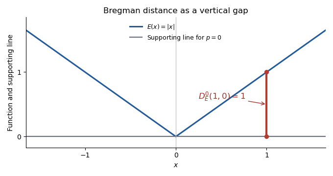
Codex 0 Created 2026-10-03 Updated 2026-10-14For , the subdifferential at zero is . Choose the allowed interior subgradient . Its supporting line is horizontal, so the Bregman distance is the vertical gap from to at the selected input:More generally, an interior choice gives . The sketch shows the particular choice .
Past exam of the mathematics course of the University of Cambridge 2016 iii Paper 326 2 ii Solution by Codex 0 Created 2026-10-03 Updated 2026-10-14
Codex 0 Created 2026-10-03 Updated 2026-10-14For the maximum-entropy regularization functional, differentiation of the scalar integrand gives . Thus the Fréchet derivative at a positive reference function is , and the stated differentiability result gives . Consequently,This is the generalized Kullback–Leibler divergence. When both functions integrate to the same mass, the last two terms cancel after integration; for probability density functions it becomes the usual Kullback-Leibler divergence. For two positive functions, adding the reverse distance givesA sufficient setting for the differentiability argument is with bounded away from zero. For nonnegative , use wherever appropriate. Positivity alone in does not automatically provide an open domain on which the Fréchet derivative exists.
Pinned article: Introduction to the OurBigBook Project
Welcome to the OurBigBook Project! Our goal is to create the perfect publishing platform for STEM subjects, and get university-level students to write the best free STEM tutorials ever.
Everyone is welcome to create an account and play with the site: ourbigbook.com/go/register. We belive that students themselves can write amazing tutorials, but teachers are welcome too. You can write about anything you want, it doesn't have to be STEM or even educational. Silly test content is very welcome and you won't be penalized in any way. Just keep it legal!
Intro to OurBigBook
. Source. We have two killer features:
- topics: topics group articles by different users with the same title, e.g. here is the topic for the "Fundamental Theorem of Calculus" ourbigbook.com/go/topic/fundamental-theorem-of-calculusArticles of different users are sorted by upvote within each article page. This feature is a bit like:
- a Wikipedia where each user can have their own version of each article
- a Q&A website like Stack Overflow, where multiple people can give their views on a given topic, and the best ones are sorted by upvote. Except you don't need to wait for someone to ask first, and any topic goes, no matter how narrow or broad
This feature makes it possible for readers to find better explanations of any topic created by other writers. And it allows writers to create an explanation in a place that readers might actually find it.
Figure 1. Screenshot of the "Derivative" topic page. View it live at: ourbigbook.com/go/topic/derivativeVideo 2. OurBigBook Web topics demo. Source. - local editing: you can store all your personal knowledge base content locally in a plaintext markup format that can be edited locally and published either:This way you can be sure that even if OurBigBook.com were to go down one day (which we have no plans to do as it is quite cheap to host!), your content will still be perfectly readable as a static site.
- to OurBigBook.com to get awesome multi-user features like topics and likes
- as HTML files to a static website, which you can host yourself for free on many external providers like GitHub Pages, and remain in full control

Figure 2. You can publish local OurBigBook lightweight markup files to either OurBigBook.com or as a static website.
Figure 3. Visual Studio Code extension installation.
Figure 5. . You can also edit articles on the Web editor without installing anything locally. Video 3. Edit locally and publish demo. Source. This shows editing OurBigBook Markup and publishing it using the Visual Studio Code extension. 
- Infinitely deep tables of contents:




All our software is open source and hosted at: github.com/ourbigbook/ourbigbook
Further documentation can be found at: docs.ourbigbook.com
Feel free to reach our to us for any help or suggestions: docs.ourbigbook.com/#contact