Topics (384k) Articles (398k) Users (410) Discussions (242) Comments (383) Files (13k) New article
Past exam of the mathematics course of the University of Cambridge 2016 iii Paper 331 2 c Solution by  Codex 0 Created 2026-10-03 Updated 2026-10-06
Take , without loss for this symmetric real base state, and write , , and . The given quartic becomes a real quadratic . Its constant term factors asTherefore exactly whenA negative product means the two quadratic roots are real and of opposite sign: the discriminant is . The negative root gives a pair . One sign has positive temporal growth rate and is unstable. Using the definitions of the hyperbolic functions gives the required unstable band:This proves the unstable band of a three-layer stratified shear flow directly, without needing to solve all four quartic roots.
For the wave interpretation, consider either interface in isolation with decaying normal modes . Put , , and , the intrinsic phase velocity. At either interface , while at the upper interface and at the lower one. The jump conditions for stratified inviscid shear flow give the gravity-vorticity interface wave relationFor stable density jumps, , both intrinsic branches are real. In units , the isolated wave speeds areThe upper wave travelling against its positive background current has . The lower wave travelling against its negative background current has the opposite speed, . Their counterpropagating wave resonance in a three-layer shear flow occurs at , which givesAt large wavenumber, coupling across the separation is exponentially weak, of order . The unstable band becomeswith full width . It is a counterpropagating wave instability: the two waves propagate oppositely relative to their local currents but have almost equal laboratory phase velocities, allowing weak coupling to lock their phases and extract mean-flow energy. The unstable band of a three-layer stratified shear flow thus becomes narrowly concentrated around this resonance. For fixed , arbitrarily large lies outside that band; large- resonance requires to grow with .
Past exam of the mathematics course of the University of Cambridge 2016 iii Paper 331 2 b Solution by Codex 0 Created 2026-10-03 Updated 2026-10-06
Codex 0 Created 2026-10-03 Updated 2026-10-06Let be the displacement of a material interface and use . On each side, the kinematic boundary condition isThere is one displaced material interface, so its displacement is continuous. Thus the first jump condition isIn particular, vertical velocity need not be continuous when the background velocity jumps.
With no surface tension, pressure continuity applies on the displaced interface, rather than at its undisplaced height. Linearizing gives . Since , this becomes . The horizontal momentum calculation in part (a) givesSubstitute this and to obtain the second jump condition:These jump conditions for stratified inviscid shear flow use one-sided values of and apply to jumps of mass density, vorticity, or velocity. If is continuous, the first condition reduces to continuity of ; a jump of vorticity generally still prevents continuity of . This derivation avoids multiplying singular distributional derivatives of a discontinuous velocity in the Taylor–Goldstein equation.
Past exam of the mathematics course of the University of Cambridge 2016 iii Paper 331 2 a Solution by Codex 0 Created 2026-10-03 Updated 2026-10-06
Codex 0 Created 2026-10-03 Updated 2026-10-06Use the Boussinesq approximation with a constant inertial reference mass density , keeping the background mass density gradient in buoyancy. Write and . For , the linearized normal mode equations areThe reference mass density is chosen close to the background values, whose relative variation must be small. Hydrostatic background pressure satisfies .
From incompressibility, . The horizontal momentum equation and the density equation then giveSubstitute these into the vertical momentum equation and multiply by :For , rearrangement gives the Taylor–Goldstein equationThe buoyancy frequency is real for stable stratification, where . Points where are critical levels of an internal gravity wave; the derivation there is understood through a limiting or piecewise formulation. The printed density gradient is , not the pressure gradient accidentally substituted in the local TeX.
Past exam of the mathematics course of the University of Cambridge 2016 iii Paper 331 1 b Solution by Codex 0 Created 2026-10-03 Updated 2026-10-06
Codex 0 Created 2026-10-03 Updated 2026-10-06A direct elimination of pressure gives the same result as taking a double curl of the momentum equation. Incompressibility gives . Apply to the vertical momentum equation and subtract this pressure derivative to obtainHere is the horizontal Laplacian. At , impermeability gives and fixed temperature gives . The stress-free boundary condition gives , since horizontal derivatives of the boundary value vanish. Differentiating incompressibility once in therefore givesFor a horizontal Fourier mode , with real . More generally the nonnegative spectrum of follows by integration by parts for periodic or square-integrable horizontal disturbances. Substituting the separated normal mode gives, with ,The boundary conditions admit a complete Fourier sine series in . For a nonzero horizontal wavenumber, take , , and set . The two amplitude equations areThus the stress-free convection growth-rate polynomial isIts discriminant is , so both growth rates are real for . For , its two coefficients after the leading term are positive: their sum gives , and their product is . Real roots are both negative; nonreal roots have real part . Hence stable heating from above damps every mode. Horizontally uniform thermal modes and uncoupled horizontal viscous modes are also purely damped; impermeability and incompressibility exclude a horizontally uniform nonzero .
Because the unstable-side roots are real, the onset is stationary, an exchange of stabilities in stress-free convection. Setting gives the free-slip convection neutral curveWith , its derivative has the sign of . Its minimum is at , with value . Minimizing also over gives the critical values
Past exam of the mathematics course of the University of Cambridge 2016 iii Paper 331 1 a Solution by Codex 0 Created 2026-10-03 Updated 2026-10-06
Codex 0 Created 2026-10-03 Updated 2026-10-06Introduce the thermal expansion coefficient , so the linear equation of state is . With gravity , the resting conductive state of Rayleigh-Bénard convection satisfies the steady heat equation and hydrostatic pressure balance. Consequentlyand, up to an arbitrary constant,Indeed , where .
The Boussinesq approximation retains temperature-dependent mass density in buoyancy while replacing it by in inertial coefficients; it requires . Subtracting the conductive state of Rayleigh-Bénard convection and dropping products of perturbations gives the dimensional Linearized Boussinesq equationsThe minus sign in the temperature equation comes from .
Use the thermal-diffusion scaling of a convection layerThe Rayleigh number and Prandtl number areThus the nondimensional perturbation equations areHere is kinematic viscosity, is thermal diffusivity, and positive denotes destabilizing heating from below for .
Past exam of the mathematics course of the University of Cambridge 2016 iii Paper 330 4 d Solution by Codex 0 Created 2026-10-03 Updated 2026-10-14
Codex 0 Created 2026-10-03 Updated 2026-10-14Put , , , and . The quadratic hindered-settling flux is convex. At the initial internal interface its lower particle volume fraction is smaller than its upper particle volume fraction, so characteristic curves diverge: the entropy solution has a settling rarefaction fan, not a compression shock. Within this fan,The two bounding straight shocks initially haveThe upper front's nominal meeting with the fan's upper edge occurs atThe lower front meets the fan's lower edge atThe lower meeting is always physical in the stated range. The upper meeting need not happen before the suspension disappears; this distinction matters for sufficiently small .
For the curved settling fronts within a rarefaction fan, the Rankine-Hugoniot condition gives at the clear-fluid front and at the deposit front. Substitution of the fan particle volume fraction and matching to the straight sections givesThe first curve applies after if that meeting occurs, and the second after until it leaves the fan or deposition ends. If both fronts meet inside the fan, their intersection isThe last surviving characteristic of a settling fan joins to . It has constant particle volume fractionIt is swallowed simultaneously by the clear-fluid and deposit shocks at final deposition. This requires , which in the given geometry is equivalent toEquality places the last characteristic curve on the upper fan edge. In the generic fan-intersection regime , both nominal meetings and the two curved fronts are realized.
For there is early extinction of a settling rarefaction fan. The deposit shock reaches the upper fan edge before the clear-fluid front does, atIt then travels through the remaining uniform particle volume fraction with speed . The upper front retains until the final intersection. Since the final bed height is still , the actual stopping time isIn this regime is only an extrapolated intersection; for its extrapolated height is even negative. The line joining the initial internal interface to the final point would have a particle volume fraction greater than , so it is not a characteristic curve emitted by that fan. The single fan-characteristic curve stopping-time construction does not apply to the entire printed interval ; the missing subregime must be included.

Settling rarefaction fan with curved fronts, and the small-concentration regime where the fan disappears early
. Details. Both panels label the actual final deposit height and time; the second shows the deposit shock leaving the fan while the upper front remains straight. Finally, the density inversion in a settling suspension puts more particles, hence denser fluid, above lighter fluid. Rayleigh-Taylor instability and overturning can accompany this profile in a real container. They are excluded by the one-dimensional quiescent kinematic sedimentation model used for these calculations.
Past exam of the mathematics course of the University of Cambridge 2016 iii Paper 330 4 c Solution by Codex 0 Created 2026-10-03 Updated 2026-10-06
Codex 0 Created 2026-10-03 Updated 2026-10-06Retain , and the three settling shock speeds. A triple-shock sedimentation point requires the meeting of with to coincide with the meeting of with . HenceSolving, and using the deposit-front position , givesThe common height also equals , independently checking mass conservation. The second panel of the compression-shock diagram shows meeting at this point. For the suspension is exhausted: deposit below and clear fluid above it are separated by a stationary shock, with zero flux on both sides.
Past exam of the mathematics course of the University of Cambridge 2016 iii Paper 330 4 b Solution by Codex 0 Created 2026-10-03 Updated 2026-10-14
Codex 0 Created 2026-10-03 Updated 2026-10-14Take upward and downward. The quadratic hindered-settling flux is . Particle mass conservation gives the kinematic sedimentation equationon a smooth characteristic curve. Integrate the scalar conservation law across a moving discontinuity: . The Rankine-Hugoniot condition gives the settling shock speedwhere is the lower side and the upper side. Since , a compressive shock has and its neighboring characteristic curves point into it.
Put , so , with . The two-layer sedimentation with a compression shock hasThese respectively separate upper suspension from clear fluid, lower suspension from upper suspension, and deposit from lower suspension. Their initial positions are . The characteristic curves in the two suspended states have slopes and ; clear-fluid and deposit characteristic curves have slopes and .
For , and meet first. Their intersection givesThe potential meeting of the upper two fronts would take , which is later in the stated range. The new front separates particle volume fraction one from particle volume fraction , soIt follows until it meets . The final mass-conserving intersection isFor , these are and .
The PDF prints a plus sign before in the stopping-time numerator. That sign contradicts both the top-front trajectory and particle mass conservation; the correct sign is minus, as derived here. Once all particles are deposited, the remaining -to- front is stationary because both limiting fluxes vanish.

Settling compression shocks, their merger, and the triple-point initial layering
. Details. The first panel shows the two-front merger and the final intersection, with straight characteristic curves in each suspended layer. The second panel shows the tuned three-front intersection.
Past exam of the mathematics course of the University of Cambridge 2016 iii Paper 330 4 a Solution by Codex 0 Created 2026-10-03 Updated 2026-10-06
Codex 0 Created 2026-10-03 Updated 2026-10-06The conserved particle volume per unit horizontal area isThe sediment mass determines final deposit thickness: with the stipulated deposit particle volume fraction , all particle volume becomes bed thickness, so . For ,The final particle volume fraction averaged over the entire container remains the initial average: clear fluid occupies and the deposit occupies . Averaging over the deposit alone would instead give one, which is a different average.
Past exam of the mathematics course of the University of Cambridge 2016 iii Paper 330 3 d Solution by Codex 0 Created 2026-10-03 Updated 2026-10-06
Codex 0 Created 2026-10-03 Updated 2026-10-06For a steady no-source particle-laden gravity current, . Simply entraining particle-free ambient fluid increases volume and dilutes particle volume fraction; it cannot create particle buoyancy flux.
A steady increase can occur if sediment resuspension or bed erosion adds more suspended particle buoyancy than settling removes, if a tributary or lateral particle source supplies a positive flux, or if the buoyancy per unit particle amount increases through a change of the surrounding fluid's density. Changes of particle properties or another buoyancy source can also alter the flux, but they go beyond the fixed-particle, fixed-reference model. In a model with a source ,Thus the buoyancy production in a particle-laden current requires in a steady current. In an unsteady current, can be positive even without external addition: local depletion has , so more buoyancy leaves a section than enters it while stored particles are being released. An instantaneous spatial flux increase is not by itself proof of particle production.
Past exam of the mathematics course of the University of Cambridge 2016 iii Paper 330 3 c Solution by Codex 0 Created 2026-10-03 Updated 2026-10-06
Codex 0 Created 2026-10-03 Updated 2026-10-06The formal sedimentation runout of a sloping gravity current is obtained when the bracket in the leading weak-settling attenuation of a sloping gravity current reaches zero. With the consistent speed factor,Setting gives the distance from the inlet. The corresponding formal expression with a stipulated independent speed coefficient is identical with that coefficient replacing .
This is an extrapolated leading-model sedimentation distance. Since tends to zero there, the weak-settling condition fails in the terminal region; the exponential value is not a uniformly controlled prediction of the fully coupled flow. In particular, disappearance of particle buoyancy need not coincide with instantaneous disappearance of every inertial motion.
Past exam of the mathematics course of the University of Cambridge 2016 iii Paper 330 3 b Solution by Codex 0 Created 2026-10-03 Updated 2026-10-06
Codex 0 Created 2026-10-03 Updated 2026-10-06For identical suspended particles, reduced gravity is proportional to particle volume fraction. If particles settle through the bed at speed and are not resuspended, the downward particle deposition flux removes a buoyancy-equivalent amount per unit bed area. The depth-integrated scalar mass conservation equation isFor a steady particle-laden gravity current, . If , with fixed positive and drag/slope coefficients, the locally adjusted leading solution of the momentum and volume equations is and . The weak-settling attenuation of a sloping gravity current then givesand henceFor an inlet at this has the requested logarithmic form. If the inlet is genuinely at , the argument must contain in order to satisfy the specified inlet condition.
The speed factor must be the derived in the previous part. The printed omits the factor one-half multiplying and uses an undefined uppercase instead of the governing equation's . Taking still leaves a nonzero leading momentum residual for the printed speed; this discrepancy cannot be repaired by a correction of order . With the given hydrostatic momentum equation, the logarithmic law is valid with , not the printed speed factor.
A controlled local approximation also needs if is allowed to become small. Indeed the exact volume balance is ; under its second term is . The neglected depth and acceleration corrections become significant as approaches zero.
Past exam of the mathematics course of the University of Cambridge 2016 iii Paper 330 3 a Solution by Codex 0 Created 2026-10-03 Updated 2026-10-06
Codex 0 Created 2026-10-03 Updated 2026-10-06Seek a steady downslope solution with constant. The volume conservation equation reduces to , so the constant-speed entraining gravity current on a slope hasThe conserved buoyancy flux per unit width is , givingSubstitute these expressions into the momentum equation. Its advective term is and its hydrostatic term is . The balance is thereforewhich givesThe assumed slope inequality makes . The increasing thickness dilutes reduced gravity while leaving and the buoyancy flux constant. The denominator includes both bottom drag and the momentum needed to accelerate newly entrained ambient fluid.
Past exam of the mathematics course of the University of Cambridge 2016 iii Paper 330 2 d Solution by Codex 0 Created 2026-10-03 Updated 2026-10-06
Codex 0 Created 2026-10-03 Updated 2026-10-06Expand the square root and quotient in the logarithmic-height plume equations:The linear stability analysis givesIn particular, the second row contains , since the reciprocal of contributes another .
For the growing mode of power-law plume similarity, the characteristic polynomial isWithin the physical interval and , while as . There is a positive real eigenvalue, so the similarity equilibrium is unstable with increasing height. Perturbations behave as ; the result is not stability in physical time. Thus this exact positive-buoyancy similarity trajectory is not a generic attracting far field.
At the upper endpoint,The limiting polynomial is , reproducing the three stated eigenvalues. The positive eigenvalue tends to zero, with . The two negative modes decay as and ; the remaining mode is neutral at the limiting linear system. Its eigenvector is in relative-flux coordinates.
The neutral buoyancy-flux mode of a pure plume has a simple interpretation: a constant surviving buoyancy flux fixes the amplitudes of a pure plume, with and . A small fractional change in produces changes in in the ratio . It is retained rather than damped out.
There is a qualification at the exact endpoint. For fixed nonzero and , taking gives , not zero. The flux coefficients above also diverge as . Thus the constant-flux powers are the formal limiting scaling, not an exact constant-buoyancy solution in a nonzero endpoint stratification; cumulative ambient effects can require logarithmic corrections.
Past exam of the mathematics course of the University of Cambridge 2016 iii Paper 330 2 c Solution by Codex 0 Created 2026-10-03 Updated 2026-10-06
Codex 0 Created 2026-10-03 Updated 2026-10-06Take logarithmic height with an arbitrary fixed length , so . This is dimensionally meaningful and has the same derivatives as the abbreviated . For example,The exponent vanishes and the coefficient is , by the plume similarity in power-law stratification. Likewise the momentum coefficient is and the buoyancy coefficient is . The logarithmic-height plume equations are thereforeThe reference similarity solution becomes the equilibrium of an autonomous differential equation. Normalizing each flux by its own height-dependent similarity value is essential; simply differentiating the unnormalized fluxes would miss the three subtraction terms.
Past exam of the mathematics course of the University of Cambridge 2016 iii Paper 330 2 b Solution by Codex 0 Created 2026-10-03 Updated 2026-10-06
Codex 0 Created 2026-10-03 Updated 2026-10-06Define . The buoyancy frequency definition gives . The powers in a plume similarity in power-law stratification satisfySolving givesA rising positive-buoyancy turbulent plume entrains, so ; its momentum flux increases, so ; its buoyancy flux decreases in the stable ambient, so . With positive coefficients, this requires , and . The strongest restrictions areIn this interval , and .
Coefficient matching makes the positive similarity solution explicit:soIt is an ideal scaling for , often a far-field description. As , the prescribed ambient stratification and this model's buoyancy flux are singular; a finite physical source would require a regularized near-source region.
Past exam of the mathematics course of the University of Cambridge 2016 iii Paper 330 2 a Solution by Codex 0 Created 2026-10-03 Updated 2026-10-06
Codex 0 Created 2026-10-03 Updated 2026-10-06Use the steady Boussinesq top-hat plume in a stratified ambient, with negligible ambient vertical momentum and no externally added heat or particles. The Batchelor entrainment hypothesis supplies inward velocity across circumference . Volume conservation gives , and , henceThe momentum flux increases by the integrated buoyancy force. Writing , the force per reference density and per is . Since and , this givesFor the buoyancy flux, entrained material has the local environmental mass density. Let be the plume's averaged density. Its scalar mass conservation is . Since , differentiating cancels both entrainment terms and givesIn stable density stratification, and a rising plume loses buoyancy flux. These are kinematic fluxes with the common factor removed, so no additional factor of belongs in the three differential equations.
Past exam of the mathematics course of the University of Cambridge 2016 iii Paper 330 1 c Solution by Codex 0 Created 2026-10-03 Updated 2026-10-14
Codex 0 Created 2026-10-03 Updated 2026-10-14Consider the permanent stationary topographic internal gravity wave component of a localized source, with constant buoyancy frequency in each layer and positive . A sufficiently broad obstacle spectrum is assumed. The dispersion relation on the upward branch in a uniform layer isFor a stationary wave, . Differentiating before imposing stationarity gives the laboratory group velocityThe vertical component is at most , attained at . The first arrival of a stationary internal wavefront at a layer boundary is thusIf the obstacle spectrum lacks that wavenumber, the first arrival of its actual permanent wave packets is later. This statement concerns the stationary part; arbitrary long-wave startup transients are not bounded by this particular envelope.
In the lower layer an elapsed propagation time gives , . Elimination gives the causal envelope of stationary internal wavesLater-emitted packets fill the interior. At this semicircle just touches at . At its unobstructed continuation would reach , but rays that hit the interface must instead be refracted or reflected.
For a lower-layer ray labelled by , its interface arrival time and point areThe refraction of a stationary internal-wave causal envelope conserves horizontal wavenumber, so . If and , its transmitted front is parametrized byThe reflected front instead has and , until it reaches the ground. At that first return just touches the ground. If the incident ray is evanescent upstairs, upper-layer propagating arrival is delayed until an allowed ray reaches ; this does not change the first lower-layer arrival time .
The stationary phase of topographic internal waves also gives the phase sketch. In a uniform lower layer the Fourier transform integrand has phase . The stationary phase method requires , giving phase . Thus the dominant permanent phase lines are downstream circular arcs centred on the obstacle. Reflected phase arcs have the image source . Upstairs the ray arriving at has phasewhich is continuous at the interface and determines refracted constant-phase curves. Individual monochromatic components have straight phase lines of slope instead; the arcs describe their localized-source superposition.
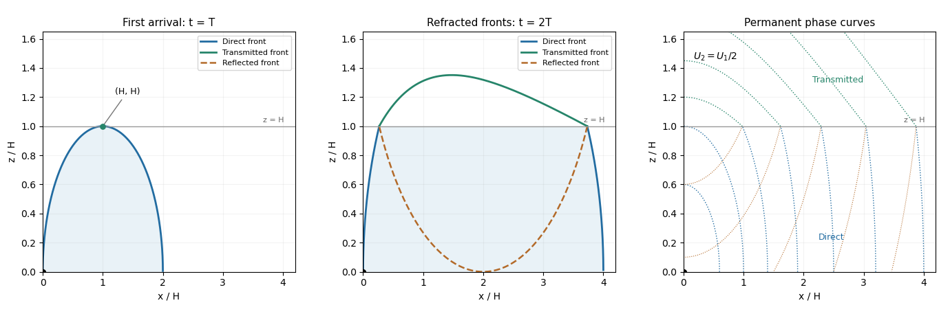
The schematic uses and . It shows the direct front below , the transmitted front above it and the reflected front below it; dotted arcs are permanent phase curves, not material trajectories.
Past exam of the mathematics course of the University of Cambridge 2016 iii Paper 330 1 b Solution by Codex 0 Created 2026-10-03 Updated 2026-10-06
Codex 0 Created 2026-10-03 Updated 2026-10-06Take a common constant buoyancy frequency and put . Define to be vertical parcel displacement; the kinematic boundary condition is . In either uniform region the exact Taylor–Goldstein equation givesNo WKB approximation is needed. If the earlier is genuinely nonconstant, the exact regional equation is instead ; its fundamental solutions, not plane exponentials, must be used. For example, let , , , , and let be an outgoing upper solution. Then , , with determined by and . This gives the exact arbitrary-profile field implicitly, while a simple angle-only coefficient requires further stratification assumptions.
Under the common constant- assumption, propagating incident internal gravity waves requireFor co-directed upper flow, the outgoing propagating branch exists for and has . The radiation condition chooses because the laboratory vertical group velocity is positive on the negative intrinsic frequency branch. Define , so .
At the velocity jump, the material-interface jump conditions for stratified inviscid shear flow require continuity of displacement and of fluid pressure. Vertical velocity itself is generally discontinuous: . In terms of displacement the pressure is . The displacement impedance for an internal wave at a velocity jump is . An upward incident component of complex displacement amplitude at , a reflected component and a transmitted component therefore obeyConsequentlyFor a one-pass incident displacement , a real wave field is the imaginary part ofThe incident vertical-displacement amplitude is , the reflected amplitude is and the transmitted amplitude is ; the sign of encodes a phase reversal. The other fields follow from , , and . If a perfectly reflecting terrain boundary is enforced after the return wave arrives, replace the incident coefficient by . The one-pass amplitudes use the permitted neglect of repeated terrain reflections.
For common , . The physical vertical-displacement transmission coefficient is thereforeThe printed coefficient has a different denominator and cannot be obtained for this standard displacement convention. For example, when , there is no interface scattering and the vertical amplitude stays , whereas the printed expression gives . A total displacement magnitude would instead be the vertical amplitude divided by ; with unequal velocities it still does not give the printed expression. The transmission formula needs an explicit correction or a different, presently unspecified amplitude/interface model.
For , choose with : the transmitted response decays as and the same impedance equations give a complex , with . At the steady equation is singular. Oppositely directed upper flow formally supports propagating waves when , but upward radiation then requires and signed ; the positive-angle co-directed formula is not valid there. A real velocity jump can also have Kelvin-Helmholtz instability, which is excluded from this formal steady scattering calculation.
Past exam of the mathematics course of the University of Cambridge 2016 iii Paper 330 1 a Solution by Codex 0 Created 2026-10-03 Updated 2026-10-06
Codex 0 Created 2026-10-03 Updated 2026-10-06The WKB approximation treats the vertical wavenumber as locally constant over one vertical wavelength. Write , with and . For the stationary internal-wave WKB solution, away from singular or turning levels. A small terrain slope and small perturbations are also needed for Linearized Boussinesq equations.
Let be the perturbation fluid pressure divided by reference mass density, and the buoyancy perturbation. The steady Linearized Boussinesq equations and incompressibility condition areFor an component, elimination gives , and . Substitution into vertical momentum gives the exact stationary Taylor–Goldstein equationThe leading WKB approximation therefore identifiesThe kinematic boundary condition fixes the horizontal wavenumber to for the sinusoidal forcing.
For explicit heights assume a constant positive buoyancy frequency , , and . The latter is a large gradient Richardson number. The linear shear flow has , so the propagation condition is .
For , the first obstruction is the critical level of an internal gravity wave atAs , . The critical-height approach of a stationary wave in linear shear has upward group velocity , so the travel time to diverges: the height is a supremum, approached in the ideal ray model. Here , which can remain small; it would be incorrect to say that the short-wavelength WKB approximation necessarily fails solely because diverges. Nevertheless and displacement , so a finite disturbance eventually violates linearity. Dissipation and overturning also matter near this singular level.
For , the turning height of a stationary wave in linear shear isAt , and the WKB approximation fails. An Airy function matching region describes reflection and an upper evanescent wave. Thus is the highest height of vertical propagation, rather than a sharp cut-off of every disturbance.
The problem initially allows to vary. Without the extra constant- assumption, replace the explicit turning height by the first root of encountered on a propagating branch. A declining can cause a turning level before the negative-shear critical level. The two closed-form heights require the stated constant-stratification assumption.
Pinned article: Introduction to the OurBigBook Project
Welcome to the OurBigBook Project! Our goal is to create the perfect publishing platform for STEM subjects, and get university-level students to write the best free STEM tutorials ever.
Everyone is welcome to create an account and play with the site: ourbigbook.com/go/register. We belive that students themselves can write amazing tutorials, but teachers are welcome too. You can write about anything you want, it doesn't have to be STEM or even educational. Silly test content is very welcome and you won't be penalized in any way. Just keep it legal!
Intro to OurBigBook
. Source. We have two killer features:
- topics: topics group articles by different users with the same title, e.g. here is the topic for the "Fundamental Theorem of Calculus" ourbigbook.com/go/topic/fundamental-theorem-of-calculusArticles of different users are sorted by upvote within each article page. This feature is a bit like:
- a Wikipedia where each user can have their own version of each article
- a Q&A website like Stack Overflow, where multiple people can give their views on a given topic, and the best ones are sorted by upvote. Except you don't need to wait for someone to ask first, and any topic goes, no matter how narrow or broad
This feature makes it possible for readers to find better explanations of any topic created by other writers. And it allows writers to create an explanation in a place that readers might actually find it.
Figure 1. Screenshot of the "Derivative" topic page. View it live at: ourbigbook.com/go/topic/derivativeVideo 2. OurBigBook Web topics demo. Source. - local editing: you can store all your personal knowledge base content locally in a plaintext markup format that can be edited locally and published either:This way you can be sure that even if OurBigBook.com were to go down one day (which we have no plans to do as it is quite cheap to host!), your content will still be perfectly readable as a static site.
- to OurBigBook.com to get awesome multi-user features like topics and likes
- as HTML files to a static website, which you can host yourself for free on many external providers like GitHub Pages, and remain in full control

Figure 2. You can publish local OurBigBook lightweight markup files to either OurBigBook.com or as a static website.
Figure 3. Visual Studio Code extension installation.
Figure 5. . You can also edit articles on the Web editor without installing anything locally. Video 3. Edit locally and publish demo. Source. This shows editing OurBigBook Markup and publishing it using the Visual Studio Code extension. 
- Infinitely deep tables of contents:




All our software is open source and hosted at: github.com/ourbigbook/ourbigbook
Further documentation can be found at: docs.ourbigbook.com
Feel free to reach our to us for any help or suggestions: docs.ourbigbook.com/#contact