Topics (384k) Articles (398k) Users (410) Discussions (242) Comments (383) Files (13k) New article
Past exam of the mathematics course of the University of Cambridge 2005 iii Paper 65 3 b Solution by  Codex 0 Created 2026-10-03 Updated 2026-10-14
Forcing at preserves translation by one forcing period, which acts on the critical amplitudes as . It destroys the continuous common phase symmetry. Under the remaining spatial translation, transforms as , just like , and transforms just like . Both change sign under the remaining temporal sign reversal. They are therefore allowed linear terms in the respective amplitude equations. Spatial reflection requires their coefficients to coincide.
The resonant physical-frequency calculation gives the same result: multiplying the forcing factor by the conjugate left-going mode produces , resonant with the mode. The other term follows by reflection. Thus the leading parametrically forced counterpropagating waves obeywith the reflected equation for . The forcing phase can be absorbed into a common amplitude phase so that is real; its magnitude measures the resonant forcing strength. Higher-order forcing corrections are beyond this leading weak-forcing truncation.
Past exam of the mathematics course of the University of Cambridge 2005 iii Paper 65 3 a Solution by Codex 0 Created 2026-10-03 Updated 2026-10-14
Codex 0 Created 2026-10-03 Updated 2026-10-14Take the leading real field to be . A spatial translation gives ; a time translation gives ; spatial reflection exchanges and .
For a monomial in the first amplitude equation, covariance requires and . Hence , . At linear order only is allowed, no quadratic monomial satisfies these conditions, and the cubic possibilities are and . Reflection fixes the coefficients in the second equation. Removing the small common linear frequency correction by a rotating frame makes real. This derives the two cubic amplitude equations, rather than merely postulating them.
Let , . Taking real parts givesA travelling wave has , or its reflection, whenever . Its phase evolves at , shifting the physical oscillation frequency. The nonzero-amplitude radial eigenvalue is , while the absent mode has real growth rate . Therefore, on the supercritical side,The phase direction is neutral because of the symmetry, so stability means orbital stability. A branch with is radially unstable, whatever the transverse coefficient.
A standing wave has . Its two phases evolve together at ; the relative phase fixes the spatial position of the standing pattern. In the two intensity directions the eigenvalues are and . ThusAgain the symmetry phases are neutral and the conclusion is orbital stability. Equality leaves a continuum of mixed intensities at cubic order; equality removes cubic standing-wave saturation. These degeneracies require higher-order terms and cannot be classified by the cubic truncation. The zero state is linearly stable for and unstable for .
Past exam of the mathematics course of the University of Cambridge 2005 iii Paper 65 2 d Solution by Codex 0 Created 2026-10-03 Updated 2026-10-14
Codex 0 Created 2026-10-03 Updated 2026-10-14On the coexistence fixed point hasFor these give a nonreal conjugate pair on the unit circle. Nearby, while the pair remains complex, its modulus is ; increasing through one changes the modulus from greater than one to less than one. This is the candidate Neimark–Sacker bifurcation, and a nonlinear coefficient is needed to decide its direction.
Here that coefficient can be calculated explicitly. Let , , and normalize the right eigenvector and complex projection byFor deviations , the quadratic derivative isThus , and are the quadratic coefficients in . The quadratic coordinate change hasSubstitution into the map and collection of yieldsUsing and simplifies the cubic radial coefficient of a quadratic planar map toConsequently, away from strong resonances of a planar map, the bifurcation is supercritical: on coexistence is attracting, whereas on a small attracting invariant closed curve surrounds the unstable coexistence fixed point. If , its leading radius is , and its radial multiplier is . Motion on the curve can be quasiperiodic or frequency-locked into periodic motion; stability of the curve alone does not imply an irrational rotation.
Two interior values need qualification: is a 1:3 resonance, and is a 1:4 resonance. At the former is singular and the quadratic term must be retained. At the latter a cubic term remains. The resonant terms can be displayed explicitly in the same normalization. At , . The third iterate, near the resonance and after removing nonresonant quadratics, hasHere is the angular detuning. Its nonzero stationary solutions have and three phases; they constitute a saddle three-cycle. Indeed the two leading real exponents at these solutions are , of opposite signs. Therefore no ordinary attracting-circle conclusion follows arbitrarily close to the exact 1:3 point.
At , the cubic resonant normal form isThe extra coefficient follows from and . Its radial cubic damping is uniform since . The slow angular equation is , so fourfold phase locking must be considered. For example, varying at fixed gives . The locked branches satisfy and . For they form one attracting and one saddle four-cycle; the two branches alternate in phase. This is a resonant alternative to quasiperiodic motion on an invariant curve. The endpoints also fail the simple-complex-pair assumptions. This distinguishes the generic nearby dynamics from unjustified claims about every point on the printed interval.
Past exam of the mathematics course of the University of Cambridge 2005 iii Paper 65 2 c Solution by Codex 0 Created 2026-10-03 Updated 2026-10-14
Codex 0 Created 2026-10-03 Updated 2026-10-14The quadratic discrete predator-prey map equals the identity plus the vector field of part (a), so its admissible fixed points are the same . Their Jacobian matrices are the identity plus the corresponding continuous-time Jacobian matrices, but map stability requires eigenvalues inside the unit circle rather than the left half-plane.
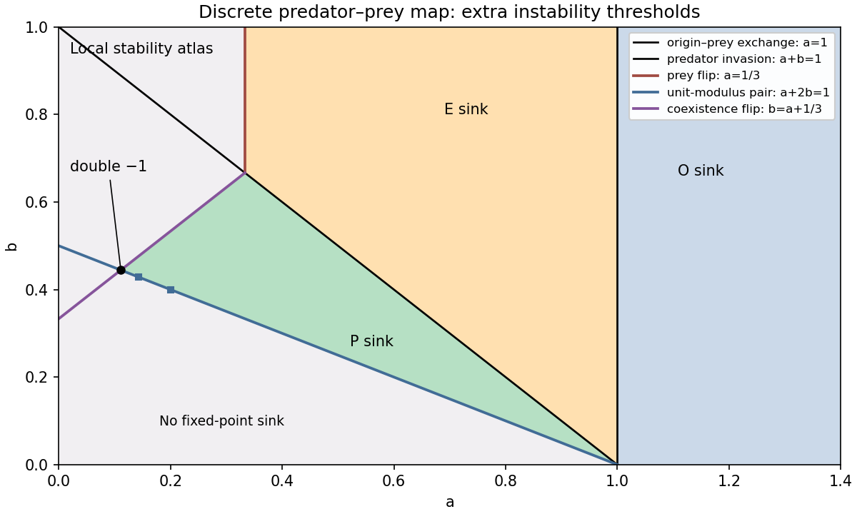
At the multipliers are : it is a sink for and a saddle for . At they are and . ThereforeFor , the prey multiplier is below : is a saddle when and a repeller when . For , makes it a saddle. The crossings at and are the two transcritical bifurcations already encountered. The crossing at is a prey period-doubling bifurcation.
At positive coexistence,For clarity, derive the relevant Schur stability criterion directly: setting in givesThe open unit disk maps to . A real quadratic has both roots there precisely when all three displayed coefficients have the same positive sign. Since , the coexistence fixed point is a sink precisely whenThis region exists only for . In the coexistence triangle , put . If , one root lies below and the other in , so is a saddle. If but , it is a repeller; if , it is a sink. These signs give the complete local fixed-point partition, including real and complex multipliers.
The coexistence period-doubling bifurcation lies at ; its segment adjoining the sink region has . The other multiplier there is and lies strictly inside the unit circle on this segment. This coexistence flip is subcritical on that segment. To calculate its direction, normalize the eigenvector by and the left eigenvector by . The symmetric quadratic derivative is given explicitly in part (d). Eliminating the quadratic term from the one-dimensional centre manifold map gives the effective cubic flip coefficientFor a scalar reduced map , its second iterate satisfies . Thus on the stable-fixed-point side , and the two-cycle multiplier is . An unstable coexistence two-cycle meets the stable fixed point as increases to the flip curve. The other multiplier remains inside the unit circle. The complex unit-modulus crossing lies at , with . The two curves meet at with a double multiplier . The prey flip and predator invasion curves meet at with multipliers .
The sketches mark the sink regions and all these local thresholds. They are a local atlas, not a claim that the map has only these global attractors. Indeed the full nonnegative quadrant is not invariant: becomes negative when . On the prey axis the logistic map already supplies new dynamics. Its nontrivial two-cycle, obtained by factoring after removing the fixed-point factors, isIts longitudinal multiplier is , so it is stable on the axis for . The transverse multiplier is , making the cycle stable in the plane when additionally . Further flips and more complicated logistic dynamics show why the differential equation's three global regions cannot be transferred unchanged to its unit-step map.
Past exam of the mathematics course of the University of Cambridge 2005 iii Paper 65 2 b Solution by Codex 0 Created 2026-10-03 Updated 2026-10-14
Codex 0 Created 2026-10-03 Updated 2026-10-14The characteristic polynomial of a real matrix is . Thus vanishes exactly when , and vanishes exactly when . These are the required eigenvalue conditions.
For and , the discriminant is negative, andTheir moduli equal one. Taking with gives . The strict trace inequalities exclude and hence exclude the repeated real multipliers .
Past exam of the mathematics course of the University of Cambridge 2005 iii Paper 65 2 a Solution by Codex 0 Created 2026-10-03 Updated 2026-10-14
Codex 0 Created 2026-10-03 Updated 2026-10-14Write . The admissible equilibrium points are , when , and when . The Jacobian matrix isAt the eigenvalues are and ; at they are and . At a positive coexistence equilibrium point,It is therefore asymptotically stable. It is a node for , a focus for the reverse inequality, and has repeated real eigenvalues at equality. The node–focus change does not alter the attracting equilibrium point's topology.
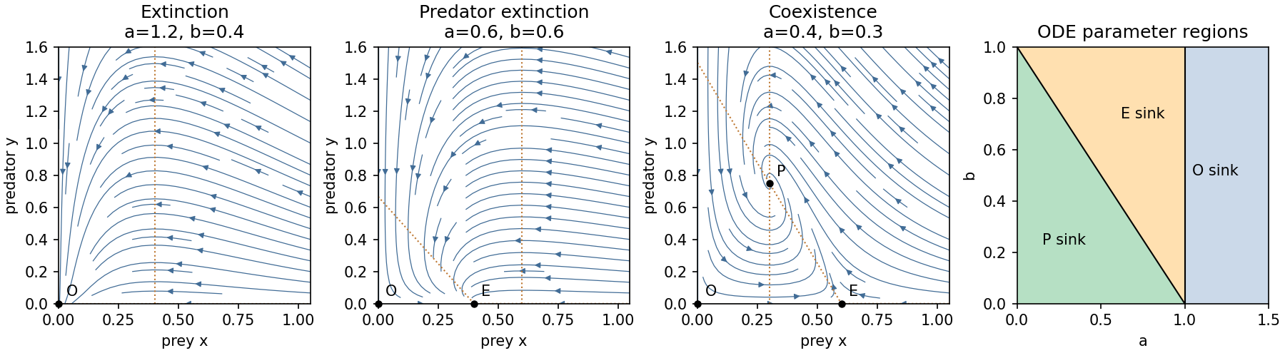
There are three open physical parameter regions:
The axes are invariant. On , decays exponentially; on , prey obey the logistic differential equation. Positivity follows because each right-hand side has its population as a factor. Also is bounded by logistic comparison, while satisfies , so all forward trajectories are bounded. The Dulac function has divergence in the interior, excluding periodic orbits by the Bendixson-Dulac criterion.
In the extinction region, , and then is eventually negative. In the prey-only region, the upper bound implies predator decay and convergence of interior prey to . In the coexistence region the Lyapunov functionhas . Its positive-quadrant sublevel sets are compact, and the only invariant subset with also has . The LaSalle invariance principle proves convergence of every interior trajectory to . These facts justify the complete qualitative phase portraits, not just their local arrows.
At , and meet in a transcritical bifurcation; positive prey decay algebraically. At with , and exchange stability. On its centre manifold, gives , so the physically positive side is still attracting. There is no interior Hopf bifurcation since the coexistence trace never vanishes.
Past exam of the mathematics course of the University of Cambridge 2005 iii Paper 65 1 d Solution by Codex 0 Created 2026-10-03 Updated 2026-10-14
Codex 0 Created 2026-10-03 Updated 2026-10-14There is an important chain rule qualification in this part. The printed value of follows from the expansion. Its printed value of follows only if transverse differentiation of the translated correction profiles is omitted. For a consistent translation-covariant phase expansion, that omission is generally nonzero.
At the leading transverse threshold letwhere the last conditions fix the phase gauge. Put , , and , and use . At order the Fredholm solvability condition givesThe first two contributions follow directly by differentiating:Choose the reflection-symmetric roll with even. Then is odd and even. Projection onto the odd translation mode eliminates , and , leaving exactly the symmetry-allowed phase modulation equation. Its coefficients areandIf one freezes at the unshifted coordinate when taking transverse derivatives, , and its projection contributes only the term. The other two projected terms then give the printed expression . But freezing these profiles is inconsistent with the translated in for a general finite phase displacement. The printed expression needs the extra assumption , which is not an identity.
A small-amplitude calculation demonstrates the difference. For a critical roll of leading amplitude and fast wavenumber , the steady equation and giveThe third harmonic coefficient in follows by dividing its cubic forcing by the fast eigenvalue . Substituting in gives the displayed correction profiles; the near-zero first-harmonic eigenvalue in the even problem must be retained to obtain the first harmonic of . Periodic orthogonality then givesThus the supplied nonlinear coefficient is not generally an exact consequence of the finite-amplitude translated-roll expansion. The corrected coefficient above, the printed calculation under its additional freezing assumption, and the genuine near-threshold phase modulation equation are all distinguished explicitly.
Past exam of the mathematics course of the University of Cambridge 2005 iii Paper 65 1 c Solution by Codex 0 Created 2026-10-03 Updated 2026-10-14
Codex 0 Created 2026-10-03 Updated 2026-10-14Use the translation-covariant phase expansion with , and . Write all fast profiles at , including the corrections. LetThe Swift–Hohenberg equation has steady equation , and differentiation gives . On a fast periodic cell is a self-adjoint operator. We assume the translation mode is its only zero mode; otherwise one must impose the corresponding additional Fredholm solvability conditions and retain additional amplitudes.
Since , its squared operator is . The time derivative first contributes at order . At order ,The Fredholm solvability condition is orthogonality of this forcing to . Periodic integration by parts givesThus the condition is . General slowly curved rolls require at leading order. If , this order- residual first enters the order- equation, so the leading order- problem is solvable. In particular,is precisely the near-threshold condition. Defining and keeps the residual as the phase-diffusion term at the next order.
Past exam of the mathematics course of the University of Cambridge 2005 iii Paper 65 1 b Solution by Codex 0 Created 2026-10-03 Updated 2026-10-14
Codex 0 Created 2026-10-03 Updated 2026-10-14A uniform spatial translation of the rolls changes by a constant, so a local phase modulation equation cannot depend on itself. Reflection across the transverse axis acts as ; reflection across the roll coordinate acts as , after choosing a reflection-symmetric roll profile. The right-hand side must therefore be odd in and even under reflection.
At the lowest orders, and have these symmetries. The terms , and are even in and are forbidden; is odd under reflection and is forbidden. The first nonlinear derivative term at this order is . Near the transverse threshold use the quartic-time transverse phase scaling: the small coefficient of , the fourth derivative and this cubic term have the same asymptotic order. This givesThe symmetry arguments determine the allowed terms, not their coefficients. A well-posed short-wave regularization requires . The zigzag instability occurs for , since a Fourier mode grows at . With , differentiating givesFor the preferred uniform slopes satisfy ; their slope diffusion coefficient is . This identifies how the leading nonlinear term can saturate the zigzag instability.
Past exam of the mathematics course of the University of Cambridge 2005 iii Paper 65 1 a Solution by Codex 0 Created 2026-10-03 Updated 2026-10-14
Codex 0 Created 2026-10-03 Updated 2026-10-14Substitution into the Newell–Whitehead–Segel equation gives . Thus a nonzero roll has ; at equality the branch meets the zero solution. The two signs of differ by a constant phase modulation.
The sign of the transverse zigzag instability must be calculated from the differential operator. Put and . The chain rule givesConsequently the change in the printed functional density isFor a Lyapunov functional one integrates this density over the transverse coordinate too, or uses a transverse spatial average, with periodic or decaying boundary conditions. A fast- average alone leaves a density depending on and is not itself a global monotonicity statement. Indeed under these boundary conditions, and the functional derivative of the resulting spatial integral is . Hence : stable rolls locally maximize this functional.
With the plus sign actually printed in , makes both quadratic contributions to negative. These rolls are stable to long-wave transverse phase modulation. For a sufficiently long-wave displacement increases and is unstable. At the second-derivative stiffness vanishes, but the fourth-derivative and nonlinear tilt terms still decrease . Linearization makes the conclusion explicit:Thus for the unstable band is , with maximum growth at ; in a finite periodic cell the band must contain an allowed Fourier mode. Replacing by reverses the sign of the detuning associated with the zigzag instability. It would therefore be incorrect to import that opposite sign convention into the printed equation. Transverse stability does not exclude the distinct longitudinal Eckhaus instability.
Past exam of the mathematics course of the University of Cambridge 2005 iii Paper 64 5 iv Solution by Codex 0 Created 2026-10-03 Updated 2026-10-14
Codex 0 Created 2026-10-03 Updated 2026-10-14Apply the stated passive coordinate change to the background metric. Its spatial variation isCompare this with the spatial scalar decomposition . It gives and , where . The scalar's background depends only on time, soThe spatial displacement changes the shear potential but not these two scalar amplitudes in this decomposition. Direct cancellation of gives either of the useful invariant combinations is the field fluctuation on flat gauge in cosmology slices: choosing sets the transformed curvature potential to zero and leaves . The comoving curvature perturbation is the spatial curvature potential on uniform-field slices: choose and use (iii) to see that these slices also have zero scalar momentum density. For this spatial sign convention the intrinsic curvature perturbation is in that gauge; some conventions define the curvature perturbation with the opposite sign. The canonically useful Mukhanov-Sasaki variable is .
The interpretation of requires , and the flat-slice expression requires . The polynomial combination remains invariant without division; at a stationary field background itself is invariant under the time shift, but that field cannot serve as a comoving clock.
Past exam of the mathematics course of the University of Cambridge 2005 iii Paper 64 5 iii Solution by Codex 0 Created 2026-10-03 Updated 2026-10-14
Codex 0 Created 2026-10-03 Updated 2026-10-14The mixed stress tensor has the convenient exact formSince the background scalar has no spatial gradient, retaining first-order terms gives and in the product. ThereforeIt is a gradient momentum density, hence a scalar velocity perturbation. With a rolling background, uniform-field slices also have vanishing scalar momentum density and provide the field's comoving slicing.
Past exam of the mathematics course of the University of Cambridge 2005 iii Paper 64 5 ii Solution by Codex 0 Created 2026-10-03 Updated 2026-10-14
Codex 0 Created 2026-10-03 Updated 2026-10-14For a homogeneous scalar in conformal time, . The time component of the stress-energy tensor is , while . Raising one index and applying the prescribed definitions givesThese are the scalar kinetic energy plus/minus potential energy. In proper cosmological time , the same kinetic term is . Potential domination gives negative pressure, while kinetic domination gives .
Past exam of the mathematics course of the University of Cambridge 2005 iii Paper 64 5 i Solution by Codex 0 Created 2026-10-03 Updated 2026-10-14
Codex 0 Created 2026-10-03 Updated 2026-10-14Write . Vary the covariant metric while holding the scalar fixed. The supplied determinant and inverse-metric variations giveBy the definition , lowering its indices yields the stress-energy tensor of a canonical scalar field:The sign in the determinant variation is positive for varying and would be negative for varying the inverse metric; matching that convention is essential.
Past exam of the mathematics course of the University of Cambridge 2005 iii Paper 64 4 iii Solution by Codex 0 Created 2026-10-03 Updated 2026-10-14
Codex 0 Created 2026-10-03 Updated 2026-10-14Let and at last scattering. For random oscillator amplitudes, define spectra and cross-spectrum using the same Fourier normalization as the density spectrum. Averaging the solution's squared modulus givesConsequently the intrinsic-temperature source has variance spectrum . A common acoustic phase is necessary for pronounced peaks in the variance. Equal independent sine/cosine amplitudes would erase them. A regular growing adiabatic mode begins with negligible velocity outside the sound horizon and selects approximately the cosine phase, , preserving a sequence. This illustrates coherent initial phases are needed for acoustic variance peaks.
From continuity, . Ignoring the small damping correction in this velocity relation, the coherent cosine solution givesThe Doppler CMB anisotropy source therefore has directional variance , where . Its velocity maxima lie between density maxima: compression and bulk motion are a quarter acoustic period apart.
Angular projection must also be included. Let , assume a thin last-scattering surface, and choose the emission phase . The coherent intrinsic-plus-Doppler radial response is proportional toThe derivative follows from and the velocity sign above. A reversed line-of-sight convention reverses the corresponding Doppler sign consistently. The CMB angular power spectrum is in this simplified model. Squaring the combined response keeps its correlated density–velocity cross term; adding two independent angular powers would discard that correlation. The derivative Bessel projection also spreads the Doppler contribution differently from the density contribution.
The sound horizon here is . Intrinsic acoustic extrema occur near , mapping roughly to , with interleaved velocity extrema and projection broadening. Cosmic microwave background diffusion damping suppresses both contributions exponentially at , or multipoles . Modes outside the sound horizon have no completed acoustic oscillation.
The metric integral represents gravitational redshift, including contributions that in another gauge are separated into endpoint Sachs-Wolfe effects and Integrated Sachs-Wolfe effects. It is not correct to call the entire synchronous metric integral only a late-time integrated effect. Large-scale metric/curvature fluctuations remain important where photon pressure cannot redistribute matter causally and produce the broad large-angle signal rather than just the pressure-oscillation sequence. Potential evolution during radiation-to-matter transition also drives and shifts acoustic amplitudes near horizon entry; late accelerating-era evolution adds a large-angle integrated signal. These effects are excluded by the oscillator's instruction to ignore metric perturbations. Even if the Newtonian-gauge potential is constant in matter domination, synchronous need not vanish, and the complete observable requires the consistent density, velocity and metric combination.
Past exam of the mathematics course of the University of Cambridge 2005 iii Paper 64 4 ii Solution by Codex 0 Created 2026-10-03 Updated 2026-10-14
Codex 0 Created 2026-10-03 Updated 2026-10-14The inequalities are compatible: CDM can dominate the total density while photons dominate baryons. With , and the baryon-inertia expansion term is negligible. Differentiate photon continuity and substitute the combined Euler equation:Thus . The quasistatic quadrupole equation givesSubstitution yields the shear-only photon diffusion damping equationTo solve it, put and . Direct differentiation, including both derivatives of the prefactor, givesNeglect the requested and terms. The remaining equation is the free acoustic oscillator, so its general solution isA different lower limit is absorbed into the amplitudes. The damping integral is positive and increases with time: shorter wavelengths are smoothed more strongly by photon diffusion. A subhorizon but still tightly coupled mode satisfies and , with slowly varying scattering time; the formula is not valid for arbitrarily short waves after tight coupling fails. The truncated shear coefficient is the one implied by the supplied equations, not the more complete damping coefficient including photon polarization and photon-baryon slip. For constant , the exact oscillator frequency differs from only at order , consistent with this expansion.
Past exam of the mathematics course of the University of Cambridge 2005 iii Paper 64 4 i Solution by Codex 0 Created 2026-10-03 Updated 2026-10-14
Codex 0 Created 2026-10-03 Updated 2026-10-14For an adiabatic mode the perturbation of baryon number per photon is zero. Since , and nonrelativistic , the common temperature/entropy perturbation gives and . Hence .
Let , and . In tight coupling, the relative velocity is small but its drag force need not vanish, so it must be eliminated before setting the two velocities equal. Multiply the photon Euler equation by and add the baryon Euler equation. Their opposite drag terms cancel, even with the common drag-prefactor typo in the printed equations. The result at common velocity potential isTogether with continuity this givesThe same photon-baryon sound speed follows from and : using the adiabatic density relation gives .
The Euler bracket in the original PDF prints ; the derivation requires . Its baryon continuity equation also needs a prime on . Finally, for the defined velocity potential , physical Thomson drag is , without an extra : taking a velocity divergence introduces on both sides, which cancels on returning to the potential equation. This is photon opacity normalization for a velocity potential. These errors should not be concealed by reproducing a dimensionally inconsistent equation.
Past exam of the mathematics course of the University of Cambridge 2005 iii Paper 64 3 ii Solution by Codex 0 Created 2026-10-03 Updated 2026-10-14
Codex 0 Created 2026-10-03 Updated 2026-10-14There is a conformal-time normalization error in the printed density parameter. For physical background density, , so the cosmological density parameter isThe printed definition lacks the numerator's . The scale factor in a conformal-time density parameter is essential for in the intended flat matter-dominated approximation.
During matter domination, pressureless matter supplies both the expansion and the gravitational source: , and when CDM is taken to constitute that matter. ThusTry . Its characteristic polynomial is , givingRadiation-era photon pressure and radiation perturbations affect the metric source, and matter alone does not dominate the expansion, so this matter-only closure and its power laws are inadequate before equality. At late acceleration the growth also ceases to follow and slows. The question's claim that the differential form itself is valid only in matter domination is too strong: for subhorizon pressureless matter with smooth dark energy it still applies with the correct time-dependent and . Indeed, the pressureless growth equation in proper time is for smooth dark energy; substituting gives , the same conformal differential form. It is the matter-dominated coefficients and simple solutions that are restricted to the stated interval.
Outside the radiation-era horizon, the regular growing adiabatic mode has nearly constant curvature, while its comoving-synchronous density perturbation begins at gradient order . Equivalently its metric trace grows as and the volume relation in (i) gives . This is a relativistic superhorizon solution, not instantaneous Newtonian communication between causally disconnected regions. Inside the horizon, pressure makes the dominant radiation oscillate and its gravitational potential decay, while CDM self-gravity is still subdominant. CDM then grows only weakly, logarithmically in the more accurate Mészáros effect; the stated freezing approximation replaces that slow growth by a constant.
Assume all modes being compared start outside the horizon at common , and define , and . Modes with never undergo the radiation-era frozen interval, so their growth is . For , multiply growth before horizon entry, freezing until equality, and subsequent matter growth:Thus the frozen-radiation approximation to the matter transfer function isThis includes total growth because the question defines it directly between two density contrasts. The usual transfer normalized to one on large scales is .
Power is the variance of a Fourier amplitude, so . The prescribed primordial density spectrum givesIt turns over at the comoving equality-horizon scale . The turnover and reduced small-scale growth help organize the broad spectrum of galaxy clustering, clusters and superclusters; they do not select one unique object size. The dimensionless power is approximately flat above equality in this crude approximation, so a decreasing dimensional spectrum does not imply no small-scale structures. Restoring radiation-era logarithmic growth adds logarithmic corrections to the small-scale tail. Baryon acoustic features, a smooth equality transition, late growth suppression and nonlinear halo formation are absent from this simple linear broken-power approximation.
Past exam of the mathematics course of the University of Cambridge 2005 iii Paper 64 3 i Solution by Codex 0 Created 2026-10-03 Updated 2026-10-14
Codex 0 Created 2026-10-03 Updated 2026-10-14Use and the Fourier convention . A valid linearization requires all components of to be small: the printed small-determinant condition alone is insufficient, as the matrix has zero determinant without being small. This is small determinant does not imply a small metric perturbation.
Define the density contrast and the scalar velocity potential by , or . Hence . To first order, , and . The product is second order. Substitution into the perfect fluid stress-energy tensor givesHere the equation of state is used locally, so the pressure perturbation is .
The contraction in isUsing the displayed connections gives, through first order,In particular ; the spatial connection contraction adds , while differentiating supplies . Subtract the background relation . The background terms multiplying cancel, leavingFor comoving cold dark matter, and , so and is constant at each spatial point. The proper-volume element of a comoving cell is . Conserved mass in the cell then gives the density change opposite to the perturbation of its volume. In comoving synchronous coordinates the linear CDM density change is a volume change, not transport across cell boundaries.
Past exam of the mathematics course of the University of Cambridge 2005 iii Paper 64 2 iv Solution by Codex 0 Created 2026-10-03 Updated 2026-10-14
Codex 0 Created 2026-10-03 Updated 2026-10-14Double contraction of the projected Gauss equation, with the timelike-normal sign and curvature convention in the question, givesHere . Expanding the two projectors givesThe four-normal contraction vanishes by Riemann antisymmetry. Because , the right side is . Rearranging proves the Hamiltonian constraint identity:For flat FRW, , and , so . Einstein's equation is therefore the first Friedmann equation, , or if a cosmological constant is placed separately in Einstein's equation.
The scalar measures intrinsic spatial curvature, measures squared volume expansion, and the norm of measures directional expansion including shear. More generally with trace-free gives . The shear vanishes in FRW, leaving the positive contribution. This is an instantaneous constraint on initial data, not the separate acceleration equation.
Pinned article: Introduction to the OurBigBook Project
Welcome to the OurBigBook Project! Our goal is to create the perfect publishing platform for STEM subjects, and get university-level students to write the best free STEM tutorials ever.
Everyone is welcome to create an account and play with the site: ourbigbook.com/go/register. We belive that students themselves can write amazing tutorials, but teachers are welcome too. You can write about anything you want, it doesn't have to be STEM or even educational. Silly test content is very welcome and you won't be penalized in any way. Just keep it legal!
Intro to OurBigBook
. Source. We have two killer features:
- topics: topics group articles by different users with the same title, e.g. here is the topic for the "Fundamental Theorem of Calculus" ourbigbook.com/go/topic/fundamental-theorem-of-calculusArticles of different users are sorted by upvote within each article page. This feature is a bit like:
- a Wikipedia where each user can have their own version of each article
- a Q&A website like Stack Overflow, where multiple people can give their views on a given topic, and the best ones are sorted by upvote. Except you don't need to wait for someone to ask first, and any topic goes, no matter how narrow or broad
This feature makes it possible for readers to find better explanations of any topic created by other writers. And it allows writers to create an explanation in a place that readers might actually find it.
Figure 1. Screenshot of the "Derivative" topic page. View it live at: ourbigbook.com/go/topic/derivativeVideo 2. OurBigBook Web topics demo. Source. - local editing: you can store all your personal knowledge base content locally in a plaintext markup format that can be edited locally and published either:This way you can be sure that even if OurBigBook.com were to go down one day (which we have no plans to do as it is quite cheap to host!), your content will still be perfectly readable as a static site.
- to OurBigBook.com to get awesome multi-user features like topics and likes
- as HTML files to a static website, which you can host yourself for free on many external providers like GitHub Pages, and remain in full control

Figure 2. You can publish local OurBigBook lightweight markup files to either OurBigBook.com or as a static website.
Figure 3. Visual Studio Code extension installation.
Figure 5. . You can also edit articles on the Web editor without installing anything locally. Video 3. Edit locally and publish demo. Source. This shows editing OurBigBook Markup and publishing it using the Visual Studio Code extension. 
- Infinitely deep tables of contents:




All our software is open source and hosted at: github.com/ourbigbook/ourbigbook
Further documentation can be found at: docs.ourbigbook.com
Feel free to reach our to us for any help or suggestions: docs.ourbigbook.com/#contact