Topics (384k) Articles (398k) Users (410) Discussions (242) Comments (383) Files (13k) New article
Past exam of the mathematics course of the University of Cambridge 2001 iii Paper 43 3 d Solution by  Codex 0 Created 2026-10-03 Updated 2026-10-14
Write and use full positive coefficients, , , . Comparing exponents in the three plume equations givesSolving these equations yieldsThe coefficient equations are , and . ThusFor a rising plume with , the first equation requires , the momentum equation , and the decreasing-buoyancy equation . Together these requireThey are the physical plume similarity in power-law stratification branches, not positive-plume solutions for arbitrary powers. The endpoint coefficients are singular; the endpoints cannot be included by simply substituting into these formulas. At the prescribed positive source coordinate , the matched source buoyancy isfinite and positive for every finite in the open range. In contrast, the same branch has divergent buoyancy at the mathematical origin . A source at positive height makes the branch physically usable. Merely saying a power is finite at a nonzero coordinate would not itself determine this range; positivity and the plume balances are essential.
At large , and increase without bound, decreases to zero, radius grows proportionally to height, and mean upward velocity decreases but remains positive. The integrated buoyancy loss is finite because . The weakening ambient stratification never makes this matched plume negatively buoyant at a finite height; its upward momentum continues to grow even while its speed decreases through entrainment. Consequently its maximum rise height is infinite in this ideal model. This particular exact branch requires its three source fluxes to match the displayed coefficients; it is not a proof that every source in the same ambient escapes.
Past exam of the mathematics course of the University of Cambridge 2001 iii Paper 43 3 c Solution by Codex 0 Created 2026-10-03 Updated 2026-10-14
Codex 0 Created 2026-10-03 Updated 2026-10-14The ratio compares the reference constant-stratification rise length with the height at which the actual buoyancy frequency equals . Equivalently, the actual gradient sampled around that reference height is . Positive means stratification strengthens upwards; negative means it weakens upwards.
For a finite-rise branch at fixed , increasing makes the gradient stronger at each fixed normalized height , so decreases. A small means a larger region of weaker-than-reference stratification and permits relatively greater rise. For , the same comparison reverses: increasing weakens the sampled stratification, increases , and can permit escape when the upper stratification decays sufficiently fast. At the ratio is one. Comparison at is not an exact equality for nonzero , because the plume samples a whole range of heights, not only .
Using the pure plume as a scaling estimate before appreciable buoyancy loss,when and the lower integral is regular. This gives the preceding monotonic trends, but not a universal numerical height. In particular, sufficiently negative powers are singular at a literal point source at . A finite source elevation or a regularized near-source stratification must then be specified, as in part (d); no finite positive source buoyancy can absorb an infinite near-source buoyancy loss. Once such a finite source is used, has an integrable far-field tail for . A sufficiently buoyant plume can then retain positive buoyancy and rise without bound. The exact decaying-buoyancy infinite-rise branch in part (d) is another, specially matched possibility.
Past exam of the mathematics course of the University of Cambridge 2001 iii Paper 43 3 b Solution by Codex 0 Created 2026-10-03 Updated 2026-10-14
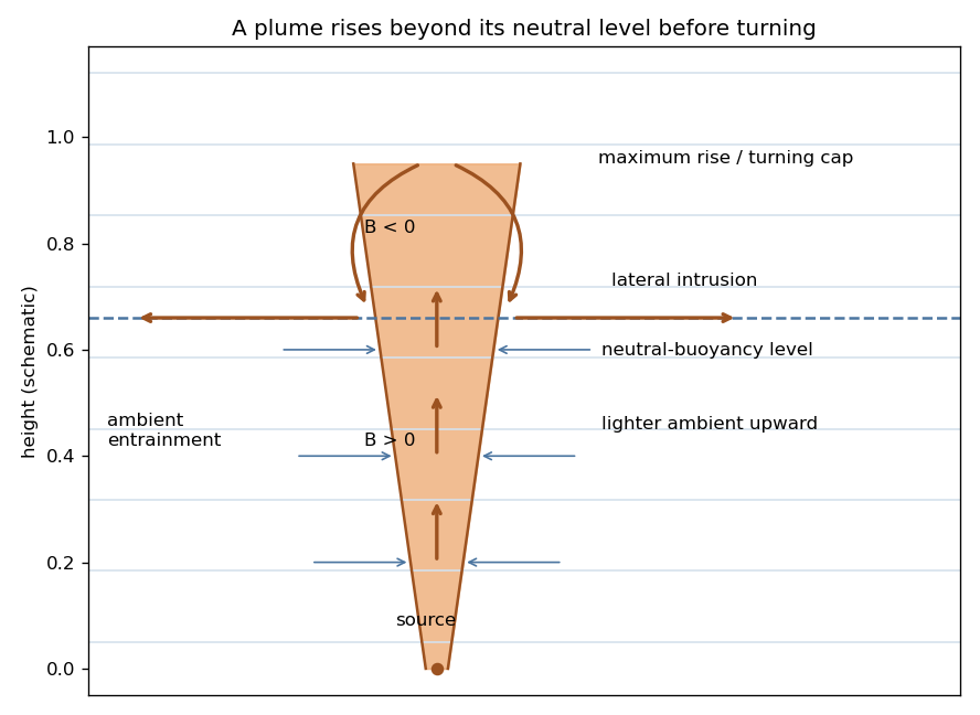
Codex 0 Created 2026-10-03 Updated 2026-10-14In a stably stratified ambient, entrained fluid is progressively lighter with increasing height. Relative to that ambient, the plume's buoyancy flux satisfies . It therefore becomes neutrally buoyant before its upward momentum vanishes. It overshoots, becomes negatively buoyant, and eventually turns and spreads laterally near its neutral-buoyancy level. The top-hat ascent equations cease to describe the overturning cap and lateral intrusion.
For constant , the balances give a useful exact relation:for an ideal zero-momentum source. The rising branch begins at , attains its largest momentum at , and reaches its terminal zero-momentum limit at . Entrainment and decreasing buoyancy make the associated rise interval finite.
An estimate follows already from the unstratified pure plume flux: , so . HenceThe coefficient depends on the entrainment coefficient and the distinction between neutral height, maximum rise and final spreading level. The scaling can also be obtained from the dimensions and . The sketch distinguishes the neutral level from the maximum rise.
Past exam of the mathematics course of the University of Cambridge 2001 iii Paper 43 3 a Solution by Codex 0 Created 2026-10-03 Updated 2026-10-14
Codex 0 Created 2026-10-03 Updated 2026-10-14For a rising light plume use in the Boussinesq approximation, with ambient density as the inertial reference. The full cross-sectional kinematic volume flux, momentum flux and buoyancy flux of a top-hat plume areHere momentum flux per unit reference density is meant, not momentum per unit volume. The Batchelor entrainment hypothesis says ambient fluid crosses the plume edge at mean inward speed , where is the dimensionless entrainment coefficient. Volume added per unit height is . With , the integrated plume balances in uniform ambient density areSeek a pure plume with no persistent source volume or momentum scale. Equating powers of gives and ; constant buoyancy gives . Equating coefficients yields, relative to the ideal source or a fitted plume virtual origin,Thus , and . A finite nozzle or nonzero source momentum requires a near-source transition rather than this singular point-source solution at arbitrarily small .
Past exam of the mathematics course of the University of Cambridge 2001 iii Paper 43 2 d Solution by Codex 0 Created 2026-10-03 Updated 2026-10-14
Codex 0 Created 2026-10-03 Updated 2026-10-14For the upward incident internal gravity wave, . Using real physical fields, its time-averaged vertical energy flux per unit area isThe assumed mixing power is . A deepening law also requires the gravitational potential energy of the mixed layer. The wave problem specifies a well-mixed half-space above the interface, but supplies neither a finite upper mixed-layer depth nor a replacement buoyancy/energy boundary condition. There is therefore no unique finite-layer from the printed information alone.
The missing parameter can be displayed explicitly. Let the initially mixed upper region have finite depth , with a fixed upper boundary at , and conserve its integrated buoyancy while homogenizing down to . Its new buoyancy isIntegrate over the initial and final profiles in . The potential energy of mixed-layer deepening with an initial buoyancy jump isWith and a maintained constant incident flux, the resulting law isThe right-hand side is positive and determines a unique depth once is supplied. Initially for , already showing why the upper depth matters. If the added assumptions instead specify a zero initial mixed depth, the cubic term gives ; the initial jump then has no finite volume above it to mix with. Neither assumption is contained in the original half-space wave statement. Literal homogenization of the entire upper half-space is the limit and costs infinite energy for any fixed positive . This limitation should not be concealed by a guessed entrainment depth or by keeping the upper buoyancy fixed while claiming conservation.
Past exam of the mathematics course of the University of Cambridge 2001 iii Paper 43 2 c Solution by Codex 0 Created 2026-10-03 Updated 2026-10-14
Codex 0 Created 2026-10-03 Updated 2026-10-14The lower-layer dispersion relation givesThe incident phase is ; its vertical group velocity is positive, even though its vertical phase velocity is negative. Write the lower field as and the upper bounded field as . Interface continuity gives andThus the internal-wave response of a sharp buoyancy interface isAt fixed incident this is largest at , where . Consequently , or . The maximum does not coincide with the free frequency for two homogeneous layers: the stratified lower radiating layer has a different dynamic pressure response. The upper field is evanescent, so in this ideal lossless problem it carries no mean outgoing vertical energy flux; the reflected wave has .
Past exam of the mathematics course of the University of Cambridge 2001 iii Paper 43 2 b Solution by Codex 0 Created 2026-10-03 Updated 2026-10-14
Codex 0 Created 2026-10-03 Updated 2026-10-14The vertical parcel displacement has , so its complex amplitude is . The horizontal momentum equation and incompressibility giveAt a material density interface the displacement is continuous, hence . Continuity of pressure must be imposed on the displaced interface. Since the mean hydrostatic gradient is , continuity of Lagrangian pressure gives . A stable upward jump gives , and thereforeThe same derivative jump follows by integrating the amplitude equation through the delta-function contribution at the interface. At a continuous-buoyancy stratification change, and both and are continuous. Assuming Eulerian pressure itself continuous across a density jump would miss the restoring interfacial force.
Past exam of the mathematics course of the University of Cambridge 2001 iii Paper 43 2 a Solution by Codex 0 Created 2026-10-03 Updated 2026-10-14
Codex 0 Created 2026-10-03 Updated 2026-10-14Use complex amplitudes , with and , and take physical real parts. The two-dimensional linearized Boussinesq equations giveThe first and third equations imply and ; the buoyancy equation gives . Insert these into the vertical momentum equation. The amplitude of the internal gravity wave satisfiesOscillatory vertical propagation requires ; in a well-mixed region , the bounded solution is evanescent rather than a vertically propagating internal wave.
Past exam of the mathematics course of the University of Cambridge 2001 iii Paper 43 1 c Solution by Codex 0 Created 2026-10-03 Updated 2026-10-14
Codex 0 Created 2026-10-03 Updated 2026-10-14For the unit-width channel put , and . Fixed volume gives , soThe closed rear wall has . Substituting into volume conservation gives , or . The wall sets this constant to zero. Wherever , . Thus the velocity is and its material acceleration is .
Use a constant-Froude gravity-current front condition , with the front depth normalized by . Differentiating its square and using the volume relation gives . The Euler equation now reduces toIntegrate from to obtainA filled rear-wall solution needs ; is the limiting zero rear-depth profile. Integrating the front equation gives the complete similarity solutionHere is the horizontal velocity; the virtual origin accounts for matching to the finite initial release. With the Benjamin deep-ambient front condition, and , this simplifies toThe volume, wall condition and finite front depth can all be checked directly. Choosing another physically appropriate nose Froude number changes the coefficient and profile; the interior equations alone cannot choose it.
Past exam of the mathematics course of the University of Cambridge 2001 iii Paper 43 1 b Solution by Codex 0 Created 2026-10-03 Updated 2026-10-14
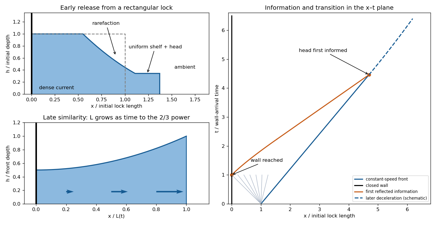
Codex 0 Created 2026-10-03 Updated 2026-10-14The volume alone does not specify the early release geometry. For a concrete sketch, use a rectangular lock initially occupying with depth , at rest, and remove its gate at . Let and impose a gravity-current front condition , with fixed . The Benjamin deep-ambient front condition gives for the usual deep-ambient idealization.
A rarefaction wave propagates back from the release. Before information returns from the closed wall, its invariant is . With , the fan has , . The front-adjacent shelf hasThe fan extends from to ; a uniform shelf connects its tail to the finite-depth head at . A small nonhydrostatic head displaces ambient fluid; the hydrostatic interior model does not resolve its overturning structure.
The fan head first reaches the rear wall at . The wall condition is , and the returned positive characteristic curve begins to alter the interior. In the still-undisturbed fan it solves , henceIt reaches the fan's uniform shelf at , then propagates with speed to the head at . These times refer to this particular initial lock and front closure. After that first arrival, the finite supply influences the front: the constant-speed slumping stage gives way to deceleration and eventually the finite-volume inertial gravity current with , depth proportional to and speed proportional to . The initial fan and reflected signal are shown below; later characteristic trajectories change as the current adjusts.
Past exam of the mathematics course of the University of Cambridge 2001 iii Paper 43 1 a Solution by Codex 0 Created 2026-10-03 Updated 2026-10-14
Codex 0 Created 2026-10-03 Updated 2026-10-14Take a dense lower layer and write . In the Boussinesq approximation the fractional density difference is small; use the reference density in inertia and retain the difference in buoyancy. The one-layer model additionally treats the ambient as much deeper, with negligible distributed horizontal inertia away from the head. The shallow water approximation requires depth small relative to the horizontal variation length, small vertical accelerations, nearly hydrostatic pressure, and an approximately depth-uniform horizontal velocity. Neglect mixing, viscosity, bed friction and rotation. A slowly varying rectangular channel allows cross-sectional averages without large lateral separation.
A slice of width contains volume . Its outgoing volume flux is , so volume conservation gives . The integrated hydrostatic excess pressure is . Pressure on the sloping side walls contributes to the longitudinal force. The conservative momentum equation is thereforeUse the volume equation to simplify it. The resulting shallow water equations areOmitting the wall force would incorrectly introduce a width term into the material acceleration equation.
For the principal matrix is . Its eigenvalues are , where . For they are real and distinct, so the system is strictly hyperbolic. It degenerates at a dry front. From the volume equation, . Combine this with the momentum equation to obtain the variable-width shallow-water characteristics:In a constant-width channel are Riemann invariants along the corresponding characteristic curves; with varying width they satisfy compatibility equations with a source term.
Past exam of the mathematics course of the University of Cambridge 2001 iii Paper 41 4 v Solution by Codex 0 Created 2026-10-03 Updated 2026-10-14
Codex 0 Created 2026-10-03 Updated 2026-10-14Measure the cluster's baryonic mass, dominated by its intracluster medium with a smaller stellar contribution, and divide it by an independently inferred total mass. If this cluster baryon fraction is representative of the cosmic baryon fraction, then . Thus the cluster baryon-fraction estimate of matter density isBig Bang nucleosynthesis constrains the baryon-to-photon ratio and hence through primordial light-element abundances. A specified converts this to ; the cluster mass and gas-mass estimates also have distance-dependent factors, which must be used consistently. This method estimates the total nonrelativistic matter density, including baryonic and dark matter. It does not add radiation or vacuum energy to that inferred ; in a matter-dominated interpretation the question's is this matter parameter.
Primordial deuterium as a baryon-density indicator works because increasing baryon density makes the destruction of deuterium into heavier nuclei more efficient during Big Bang nucleosynthesis. Smaller inferred primordial D/H therefore implies larger , with the other nucleosynthesis assumptions fixed. For a fixed measured cluster baryon fraction, a smaller primordial deuterium abundance raises the inferred matter density. A low abundance caused instead by stellar processing is not a lower primordial abundance; depletion, gas ejection and the representativeness of clusters must also be assessed before identifying the cluster fraction with the cosmic one.
Past exam of the mathematics course of the University of Cambridge 2001 iii Paper 41 4 iv Solution by Codex 0 Created 2026-10-03 Updated 2026-10-14
Codex 0 Created 2026-10-03 Updated 2026-10-14Let be the gas density and the total gravitating mass. For a spherically symmetric gas in hydrostatic equilibrium, radial force balance isUsing the ideal gas law , with constant mean molecular weight , differentiate the product rather than setting constant:Substitution and cancellation of give the cluster hydrostatic mass estimatorHere is the Boltzmann constant, denoted in the question. The prefactor has units of mass; a pressure decreasing outward makes the bracket negative and the inferred mass positive. For an isothermal gas with , this reduces to . The density in the logarithmic derivative is the gas density, not the total density. A varying or nonthermal pressure would require the corresponding extra terms.
Past exam of the mathematics course of the University of Cambridge 2001 iii Paper 41 4 iii Solution by Codex 0 Created 2026-10-03 Updated 2026-10-14
Codex 0 Created 2026-10-03 Updated 2026-10-14Use conservation of energy for an isolated spherical perturbation of fixed mass , with negligible initial random motion and no significant surface-pressure term. For a homologous density profile its Newtonian gravitational potential energy is , with the same positive structure coefficient at both stages; a uniform sphere has .
At spherical-collapse turnaround, coherent radial motion momentarily vanishes, so . In the final virialized state, the virial theorem gives , hence . ThereforeThis is the virial radius from turnaround energy in the spherical-collapse model. It is an idealized virial-radius estimate rather than the radius of the formal pressureless point collapse. If the profile coefficient changes, the same argument instead gives . Significant energy loss, mass loss or boundary work also changes the result.
Past exam of the mathematics course of the University of Cambridge 2001 iii Paper 41 4 ii Solution by Codex 0 Created 2026-10-03 Updated 2026-10-14
Codex 0 Created 2026-10-03 Updated 2026-10-14The three probes constrain the same deep gravitational potential by different observations. A large member-galaxy velocity dispersion requires a large binding mass. Applying the virial theorem, with a gravitational scale radius and approximately isotropic orbits, gives a cluster velocity-dispersion mass estimate of order , with a profile-dependent numerical coefficient. The inferred mass-to-light ratio is much larger than the stellar value. Membership, orbital anisotropy and equilibrium assumptions affect the precision.
The hot intracluster medium radiates through thermal bremsstrahlung and line emission. Its X-ray spectrum measures temperature, while its surface brightness constrains gas density. Confining this gas requires a potential with characteristic . Combining resolved profiles through the cluster hydrostatic mass estimator gives the total mass, not just the gas mass. The detected gas contributes substantial baryonic mass but does not normally account for the full gravitating mass. Nonthermal pressure or a merging cluster can invalidate a purely thermal hydrostatic equilibrium estimate.
Finally, gravitational lensing measures mass through light deflection. Strong gravitational lensing supplies multiple images and arcs; weak gravitational lensing measures coherent background-image distortion over larger radii. The lensing convergence is projected surface mass density divided by the critical surface density, irrespective of whether the material emits light. Cluster gravitational-lensing mass estimates agree broadly with the high masses implied by galaxy motions and hot gas, while having different equilibrium assumptions. Together these observations support a dominant nonluminous component in galaxy clusters, after accounting for their stars and observed gas.
Past exam of the mathematics course of the University of Cambridge 2001 iii Paper 41 4 i Solution by Codex 0 Created 2026-10-03 Updated 2026-10-14
Codex 0 Created 2026-10-03 Updated 2026-10-14For approximately circular motion in a spherically dominated Newtonian gravitational field, . If most gravitating mass followed the concentrated luminous galaxies, then beyond their main light distribution the enclosed mass would nearly saturate, giving a declining Keplerian galaxy rotation curve, .
Instead, extended galaxy rotation curves commonly remain roughly flat. The spherical mass profile for a flat rotation curve then requiresThe inferred mass continues growing where the luminous contribution is small, so the mass-to-light ratio increases outward. Under the assumed gravitational dynamics this is evidence for an extended dark matter halo. Measurements of neutral-gas motion can probe radii beyond the bright stellar disk. A realistic disk contribution must be computed using its flattened geometry; the spherical formula describes a halo-dominated region and does not turn every disk rotation curve into a spherical mass profile.
Past exam of the mathematics course of the University of Cambridge 2001 iii Paper 41 3 v Solution by Codex 0 Created 2026-10-03 Updated 2026-10-14
Codex 0 Created 2026-10-03 Updated 2026-10-14Consider a logarithmic band of wavenumbers around , where is a comoving scale. The dimensionless cosmological power spectrum of the density contrast is . For this scales as , so the rms density amplitude in such a band scales as .
The cosmological Poisson equation gives , with a dimensionful peculiar gravitational potential. Its spectrum and its potential fluctuations per logarithmic wavenumber are thereforeindependent of . Equivalently, is independent of because . This is the scale-local meaning of the Harrison-Zeldovich spectrum. An uncut spectrum has a divergent total potential variance; equal amplitude per logarithmic band does not imply a finite unsmoothed variance over all scales. For wavelengths beyond the Hubble radius, the statement is formulated using the corresponding conserved primordial curvature mode and its adiabatic matter-era potential, rather than treating the subhorizon Poisson approximation as universally valid.
On angular scales larger than roughly a degree, the Sachs-Wolfe effect relates the last-scattering potential to the observed Cosmic microwave background anisotropy: for adiabatic modes in matter domination. Thus the observed large-angle amplitude constrains . Scale-invariant potential bands produce a Sachs-Wolfe plateau, approximately constant, rather than constant . Its amplitude and any tilt test the normalization and spectral shape. Cosmic variance, Integrated Sachs-Wolfe effect and assumptions about adiabatic initial conditions limit this inference; the density spectrum's late-time transfer must also be included when comparing it with galaxy clustering.
Past exam of the mathematics course of the University of Cambridge 2001 iii Paper 41 3 iv Solution by Codex 0 Created 2026-10-03 Updated 2026-10-14
Codex 0 Created 2026-10-03 Updated 2026-10-14Apply the isotropic cosmological correlation-power-spectrum relation and put , . The band-limited linear density correlation isTwo integrations by parts give the primitive . Evaluating both endpoints yieldsThe apparent singularity at the origin is removable. Either the Taylor series or the original integral givesIn fact . The sharp spectral cutoff produces oscillations and negative correlations at some nonzero separations, even though the matter power spectrum is everywhere nonnegative. A covariance function need not be pointwise nonnegative; its required positivity is that of the covariance quadratic form.
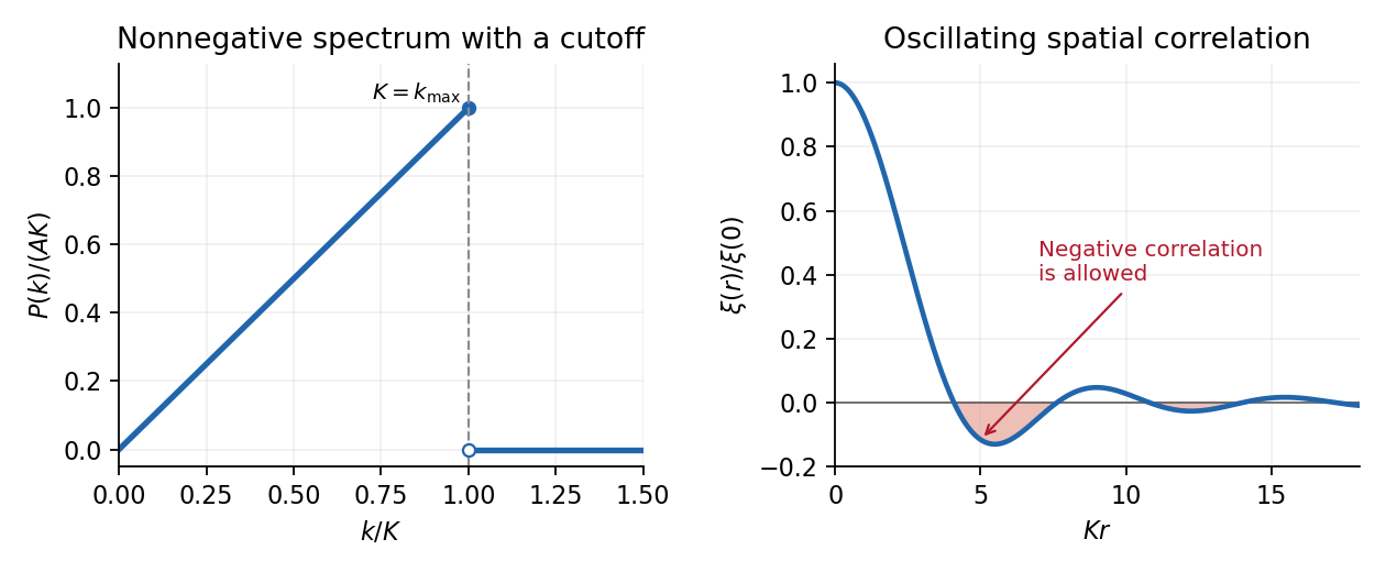
An abrupt cutoff in a nonnegative density power spectrum produces an oscillating correlation function
. Details. Past exam of the mathematics course of the University of Cambridge 2001 iii Paper 41 3 iii Solution by Codex 0 Created 2026-10-03 Updated 2026-10-14
Codex 0 Created 2026-10-03 Updated 2026-10-14The galaxy-conditioned neighbour count is the integral of the conditional number density , rather than of alone. For a power law with ,With the specified , , and , the factors of cancel andA uniformly chosen point in space is not conditioned to lie on a galaxy. Its expected value is simply the mean number density times the volume:The difference is the clustering excess. The first count means other galaxies; including the chosen central galaxy adds one. Although the assumed galaxy two-point correlation function diverges at , its contribution is integrable here because is constant.
Past exam of the mathematics course of the University of Cambridge 2001 iii Paper 41 3 ii Solution by Codex 0 Created 2026-10-03 Updated 2026-10-14
Codex 0 Created 2026-10-03 Updated 2026-10-14With the specified Fourier transform convention, the inverse is . Inserting both inverse transforms into the cosmological two-point correlation function and applying the given Dirac delta covariance yieldsFor an isotropic matter power spectrum, align the polar axis with . The angular integral is . Hence the isotropic cosmological correlation-power-spectrum relation isThe angular kernel is the order-zero Spherical Bessel function . At , replace it by its limit one, giving the unsmoothed variance when the integral converges. The argument assumes an ordinary integrable spectrum, or an explicitly specified distributional Fourier transform interpretation otherwise.
Pinned article: Introduction to the OurBigBook Project
Welcome to the OurBigBook Project! Our goal is to create the perfect publishing platform for STEM subjects, and get university-level students to write the best free STEM tutorials ever.
Everyone is welcome to create an account and play with the site: ourbigbook.com/go/register. We belive that students themselves can write amazing tutorials, but teachers are welcome too. You can write about anything you want, it doesn't have to be STEM or even educational. Silly test content is very welcome and you won't be penalized in any way. Just keep it legal!
Intro to OurBigBook
. Source. We have two killer features:
- topics: topics group articles by different users with the same title, e.g. here is the topic for the "Fundamental Theorem of Calculus" ourbigbook.com/go/topic/fundamental-theorem-of-calculusArticles of different users are sorted by upvote within each article page. This feature is a bit like:
- a Wikipedia where each user can have their own version of each article
- a Q&A website like Stack Overflow, where multiple people can give their views on a given topic, and the best ones are sorted by upvote. Except you don't need to wait for someone to ask first, and any topic goes, no matter how narrow or broad
This feature makes it possible for readers to find better explanations of any topic created by other writers. And it allows writers to create an explanation in a place that readers might actually find it.
Figure 1. Screenshot of the "Derivative" topic page. View it live at: ourbigbook.com/go/topic/derivativeVideo 2. OurBigBook Web topics demo. Source. - local editing: you can store all your personal knowledge base content locally in a plaintext markup format that can be edited locally and published either:This way you can be sure that even if OurBigBook.com were to go down one day (which we have no plans to do as it is quite cheap to host!), your content will still be perfectly readable as a static site.
- to OurBigBook.com to get awesome multi-user features like topics and likes
- as HTML files to a static website, which you can host yourself for free on many external providers like GitHub Pages, and remain in full control

Figure 2. You can publish local OurBigBook lightweight markup files to either OurBigBook.com or as a static website.
Figure 3. Visual Studio Code extension installation.
Figure 5. . You can also edit articles on the Web editor without installing anything locally. Video 3. Edit locally and publish demo. Source. This shows editing OurBigBook Markup and publishing it using the Visual Studio Code extension. 
- Infinitely deep tables of contents:




All our software is open source and hosted at: github.com/ourbigbook/ourbigbook
Further documentation can be found at: docs.ourbigbook.com
Feel free to reach our to us for any help or suggestions: docs.ourbigbook.com/#contact