Topics (384k) Articles (398k) Users (410) Discussions (242) Comments (383) Files (13k) New article
Past exam of the mathematics course of the University of Cambridge 2001 iii Paper 52 5 b Solution by  Codex 0 Created 2026-10-03 Updated 2026-10-14
Use a globally coupled underdominant metapopulation with equal habitat sizes:Symmetry preserves a common frequency in the initially habitats and in the initially habitats. With , the equations reduce exactly toThe maximum positive selection rate is at . Comparing it with the worst outward migration flux gives a sufficient barrier condition . A slightly stronger optimized condition follows from maximizing the per-capita restoring term over : its maximum is at .
Indeed, on , with , . On , with , . The other two edges point inward as well. The invariant-rectangle criterion for underdominant coexistence therefore gives the explicit robust conditionsStarting from the specified pure habitats, the populations then remain in , . Their global frequency lies between and , so neither allele fixes. This is a sufficient condition, not a claim that the bound is sharp. If or , the population is already fixed; if , any mixture of the two pure habitat types persists.
The exactly balanced case illustrates why robustness and the prescribed trajectory differ. When , symmetry forces andFor its heterogeneous limiting state isHere , so the full Jacobian matrix has diagonal entries and off-diagonal entries . Its two full-system eigenvalues are and : the symmetric underdominant two-cluster equilibrium is robustly attracting only for . For larger migration the exactly symmetric initial condition can still avoid fixation, eventually approaching the spatially uniform frequency when , but the symmetry-broken mean-frequency mode is unstable. A finite population with genetic drift need not maintain deterministic coexistence indefinitely.
Past exam of the mathematics course of the University of Cambridge 2001 iii Paper 52 5 a Solution by Codex 0 Created 2026-10-03 Updated 2026-10-14
Codex 0 Created 2026-10-03 Updated 2026-10-14Let be the allele frequency of , with random mating and sufficiently large population size to neglect genetic drift. The Hardy-Weinberg proportions before selection are . Write the three genotype fitnesses as , with smaller than either homozygote value. After one viability-selection generation,ConsequentlyPut , . The underdominant allele-frequency dynamics has stable fixation states zero and one, separated by the unstable thresholdBelow it decreases to allele fixation of ; above it increases to fixation. Exactly at the threshold the deterministic frequency remains balanced, but any perturbation selects a side. This is underdominance, or heterozygote disadvantage, rather than balancing selection from heterozygote advantage.
Past exam of the mathematics course of the University of Cambridge 2001 iii Paper 52 4 c Solution by Codex 0 Created 2026-10-03 Updated 2026-10-14
Codex 0 Created 2026-10-03 Updated 2026-10-14The high-contact assumptions give away from a degeneracy. Since , perturbing the larger eigenvalue in the assortatively mixed two-risk-group SIS model givesFor the biologically useful high-risk-core regime , put . Substituting and into the two equilibrium equations givesThus the group susceptible fractions and their population-weighted total areThe small-core SIS endemic expansion shows why the homogeneous SIS susceptible fraction relation fails for a mixed population: as the high-risk fraction tends to zero, while . A small high-risk core sustains infection even though almost everyone in the population remains susceptible. Even need not equal at first order.
For completeness, if with a fixed gap from threshold, small gives disease-free equilibrium and total susceptibility one. If , the low-risk group already sustains infection. Put and let be the positive root of . The first-order coefficients areAgain it tends to rather than . These regular expansions require fixed nonzero gaps. At the spectral splitting is generally order ; at , low-risk infection is also order , so a regular first-order Taylor expansion is inappropriate. An exact endemic replacement for the scalar identity is that the susceptible-weighted next-generation matrix has spectral radius one.
Past exam of the mathematics course of the University of Cambridge 2001 iii Paper 52 4 b Solution by Codex 0 Created 2026-10-03 Updated 2026-10-14
Codex 0 Created 2026-10-03 Updated 2026-10-14Use an assortatively mixed two-risk-group SIS model with equal per-person recovery rate . Let be infectious proportions in groups of sizes . Let be their fixed contact rates and the transmission probability per contact. Suppose a small fixed fraction of high-risk contacts is with the low-risk group. Contact reciprocity in a two-group epidemic requiresFor sufficiently small , both groups make most contacts within their own group, and the total cross-group contacts are of order . Define , , and . The forces of infection giveHere and hold in the small- regime. High-risk per-person cross contact is order one but its group size is order ; low-risk per-person cross contact is order . These distinctions are needed to count each cross-group partnership consistently.
Linearize about the disease-free state. In infectious fractions the transmission matrix isIn infected-individual counts the next-generation matrix is insteadThe count and fraction formulations are related by a diagonal change of coordinates, so their eigenvalues coincide. The basic reproduction number is the spectral radius , not an average of the two group reproduction numbers. The larger real eigenvalue isThis model makes a particular reciprocal mixing convention explicit; different defensible contact laws can change the first-order coefficients.
Past exam of the mathematics course of the University of Cambridge 2001 iii Paper 52 4 a Solution by Codex 0 Created 2026-10-03 Updated 2026-10-14
Codex 0 Created 2026-10-03 Updated 2026-10-14Let be the infectious proportion in a closed population. With homogeneous frequency-dependent transmission rate and recovery rate , the SIS model isThe basic reproduction number is the expected number of secondary infections produced by a typical newly infected individual in an otherwise susceptible population under the specified contact conditions. Here the infectious duration has mean , so .
For the attracting endemic equilibrium has . The homogeneous SIS susceptible fraction is thereforeFor the physical equilibrium is disease-free, , . At equality approach to zero is algebraic. Thus is an endemic relation, not a formula demanding more than one susceptible person per person below the invasion threshold.
Past exam of the mathematics course of the University of Cambridge 2001 iii Paper 52 1 b Solution by Codex 0 Created 2026-10-03 Updated 2026-10-14
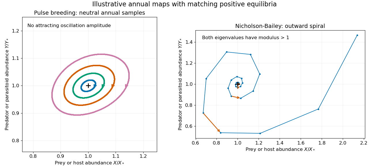
Codex 0 Created 2026-10-03 Updated 2026-10-14For the adult-survival annual pulse-breeding predator-prey model, a positive annual fixed point exists when and :At this point the Jacobian matrix isIf , the two eigenvalues are a complex conjugate pair of moduli one. The annual samples show linearly neutral seasonal oscillations. If , they form a reciprocal negative real pair and the fixed point is a saddle fixed point of a map. Equality at four is a degenerate boundary needing nonlinear analysis. For replacement rather than surviving adults the same calculation gives trace and determinant one.
The absence of an attracting annual cycle is stronger than a linear observation. Put , . The update becomesIt is the composition of two nonlinear shear maps, each of determinant one: an area-preserving seasonal predator-prey map. No isolated positive periodic orbit has an open attracting basin. Neutral linear oscillations alone also do not prove nonlinear stability at every resonance. In particular, this density-independent model does not select an asymptotically stable oscillation amplitude.
The Nicholson-Bailey model instead counts parasitoid offspring from attacked hosts:Its positive equilibrium has and . Its Jacobian matrix hasSince the determinant exceeds one while the positive trace is below two, the eigenvalues are complex with moduli greater than one: instability of the Nicholson-Bailey equilibrium produces outward oscillations near it. The two maps share an exponential prey-survival factor but have different reproduction laws and stability properties.
Past exam of the mathematics course of the University of Cambridge 2001 iii Paper 52 1 a Solution by Codex 0 Created 2026-10-03 Updated 2026-10-14
Codex 0 Created 2026-10-03 Updated 2026-10-14Use an annual pulse-breeding predator-prey model. Let be the abundances just after reproduction, and let the year have length . Between breeding pulses, assume mass-action predation, natural mortality rates , and no reproduction:Solving the predator equation and inserting it into the prey equation gives the pre-breeding abundancesSuppose reproduction multiplies surviving prey by and adds offspring per surviving predator. Retaining the surviving adults gives , . Define , , and . The resulting difference equations areThus offspring depend on prey available at the end of the year, not on the number killed during the year. The adult-survival convention is part of the model; if breeding replaces all adults, use instead. Both are consistent pulse models under their respective life-history assumptions.
Past exam of the mathematics course of the University of Cambridge 2001 iii Paper 51 3 d Solution by Codex 0 Created 2026-10-03 Updated 2026-10-14
Codex 0 Created 2026-10-03 Updated 2026-10-14At the saddle equilibrium , put . The two eigenvalues and saddle index areOn the nearby saddle-loop curve, . Therefore , with the more explicit expansionThe positive saddle quantity makes the loop repelling. In a transverse section its leading return map has the form ; its derivative grows without bound as . This is the mechanism by which a positive saddle quantity makes a nearby saddle loop repelling. It agrees with the repelling periodic orbit coming from the subcritical Hopf bifurcation, rather than predicting an attracting cycle at the collision.
Past exam of the mathematics course of the University of Cambridge 2001 iii Paper 51 3 c Solution by Codex 0 Created 2026-10-03 Updated 2026-10-14
Codex 0 Created 2026-10-03 Updated 2026-10-14Along a perturbed saddle loop the incoming and outgoing endpoints have the same Hamiltonian value. Integrating and evaluating the leading integral on the conservative homoclinic orbit givesOn the upper half of the loop and . The lower half makes an equal contribution, soThese homoclinic integrals for a quadratic-force oscillator give the simple first-order splitting zero , since . The Melnikov energy-balance method therefore yields the leading global bifurcation curveThis is an asymptotic curve near the double-zero point, not an exact finite-parameter identity. More precisely, time reversal preserves the loop condition. The smooth curve selected by its simple splitting zero is even in , giving and hence for fixed scaled .
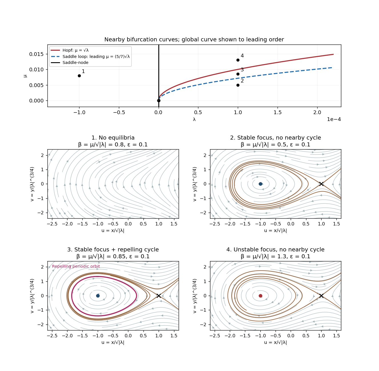
Between the saddle-loop curve and , a stable focus is surrounded by the repelling periodic orbit created at the subcritical Hopf bifurcation. As decreases, this orbit grows until it reaches the saddle. Below the saddle-loop curve there is a stable focus and a saddle, but no nearby cycle. Above the Hopf curve there is an unstable focus and a saddle, with no nearby cycle. At the global curve the saddle separatrices form the repelling loop. Under the stipulated absence of further bifurcations, these are the distinct nearby regions in the earlier sketch; no extra remote phase structure is being inferred from the leading-order calculation.
Past exam of the mathematics course of the University of Cambridge 2001 iii Paper 51 3 b Solution by Codex 0 Created 2026-10-03 Updated 2026-10-14
Codex 0 Created 2026-10-03 Updated 2026-10-14Substitution of the weighted scaling and givesThe derivative of the candidate Hamiltonian isThus is a conserved quantity at . For put . The conservative equilibrium point is a center with , and is a saddle equilibrium with saddle-loop energyThe closed component of a level between these energies surrounds the center. At ,is the homoclinic orbit, with left turning point . The upper branch is traversed to the right and the lower branch to the left. Levels above the barrier have escaping trajectories; the saddle level also has unbounded branches to the right. For the two critical points coalesce; for the potential is monotone and there is no center or saddle loop.
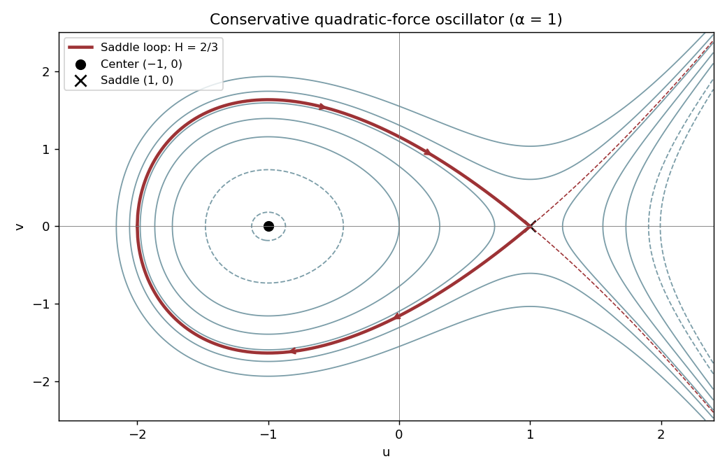
Hamiltonian level curves and the conservative saddle loop for alpha equal to one
. Details. Past exam of the mathematics course of the University of Cambridge 2001 iii Paper 51 3 a Solution by Codex 0 Created 2026-10-03 Updated 2026-10-14
Codex 0 Created 2026-10-03 Updated 2026-10-14The equilibrium points satisfy , . For there are none. For set . The Jacobian matrix isThe positive equilibrium point is always a saddle equilibrium. At the determinant is , so it is stable for and unstable for . The discriminant distinguishes a node from a focus; its zero does not destroy hyperbolicity and is not another local bifurcation curve.
The local bifurcation curves areAt the linearization has a double zero eigenvalue and is nilpotent, giving a Bogdanov–Takens bifurcation. For on , solving the local center manifold gives , displaying the saddle-node bifurcation. For the nonsaddle branch born at positive is attracting; for it is repelling. On the Hopf curve the angular frequency is . The permitted subcritical Hopf bifurcation creates a repelling periodic orbit on the stable-focus side .
A local analysis alone does not say how far that periodic orbit extends. The global calculation below supplies the additional division of the stable-focus region. The complete nearby phase portraits and the leading global curve are shown together here. The flow has no closed periodic orbit, since a closed orbit would have index one and hence enclose an equilibrium point.
Past exam of the mathematics course of the University of Cambridge 2001 iii Paper 51 2 c Solution by Codex 0 Created 2026-10-03 Updated 2026-10-14
Codex 0 Created 2026-10-03 Updated 2026-10-14On the nonzero stationary branch of five-mode magnetoconvection, put and . The temperature equations first give and . The magnetic equations then giveDivide the steady first equation by and substitute these expressions. The exact branch isExpanding at givesNear the required amplitude restriction ensures . For , , so the paired equilibrium points emerge in the forward direction . For fixed and small , the pitchfork reversal near geometric ratio two in magnetoconvection occurs atThis follows by expanding the exact zero-slope equation . Above this value the branch initially runs backwards into ; at there is no reversal. This is a degenerate pitchfork bifurcation at , not a conclusion that every emerging state is stable. If , the center-direction cubic term has the opposite sign to : the forward branch is locally attracting and the backward branch repelling. If , an unstable transverse mode remains.
For the nearby geometry, the next coefficient is , which is negative near the reversal. Thus a small positive produces a nearby maximum of at ; this fold approaches the pitchfork as . Once the small-amplitude branch is backward. The exact formula eventually grows like , so a backward branch must turn at a finite amplitude, potentially outside the small-amplitude expansion.
Past exam of the mathematics course of the University of Cambridge 2001 iii Paper 51 2 b Solution by Codex 0 Created 2026-10-03 Updated 2026-10-14
Codex 0 Created 2026-10-03 Updated 2026-10-14At conduction, and have stable eigenvalues and . The remaining linearization on isIts characteristic polynomial is , whereConsequently the steady threshold is . The symmetry , with unchanged, gives a generic pitchfork bifurcation, whose forward or backward direction is determined below. At threshold the other two critical-block eigenvalues satisfy , where . They are stable if ; if there is already one unstable transverse direction. Degenerate zero cubic slope requires higher-order analysis and is not a generic pitchfork.
At a Hopf bifurcation, , . Solving the coefficient equation givesFor physical the oscillatory threshold therefore exists exactly when and . The conduction double-zero criterion for five-mode magnetoconvection givesAt this Bogdanov–Takens bifurcation, the polynomial is and the zero eigenspace is one-dimensional. For conduction first loses stability at the steady threshold; for it first loses stability at . For no positive- double-zero or oscillatory threshold exists. These conclusions also follow from the Routh-Hurwitz stability criterion, and . The Hopf bifurcation is transversal since ; its nonlinear criticality is not required by this linear onset calculation.
Past exam of the mathematics course of the University of Cambridge 2001 iii Paper 51 2 a Solution by Codex 0 Created 2026-10-03 Updated 2026-10-14
Codex 0 Created 2026-10-03 Updated 2026-10-14Use the Galerkin method, rather than pointwise equality: products generate harmonics outside the retained five-dimensional space. Put , , and denote the five prefactors byThe retained streamfunction is , the retained temperature perturbation is , and the retained magnetic-flux perturbation is . These satisfy all the stated boundary conditions. Let , the streamfunction advection bracket. Orthogonality of the sine and cosine modes gives the following coefficients of the retained harmonics:For example the contribution to the temperature bracket is . The magnetic bracket follows by writing : and . These identities exhibit both the retained terms and discarded harmonics.
Before rescaling time, the projected coefficient equations areSubstitute the prefactors and divide time derivatives by . With , and , the resulting five-mode vertical-field magnetoconvection equations areHere primes denote differentiation in . The factor is , which checks the magnetic nonlinear sign. There is a terminology qualification in the source: on this thermal diffusion time scale, its is the magnetic-to-thermal diffusivity ratio . The conventional magnetic Prandtl number is , where is the Prandtl number. The displayed equations and subsequent calculation use the source's unchanged.
Past exam of the mathematics course of the University of Cambridge 2001 iii Paper 51 1 f Solution by Codex 0 Created 2026-10-03 Updated 2026-10-14
Codex 0 Created 2026-10-03 Updated 2026-10-14To include the stable-variable lag in nilpotent center-manifold reduction, let . Invariance of the center manifold requiresFor the homogeneous polynomial , comparison of coefficients successively givesOnly is needed for the requested cubic normal form. The reduced first equation has ; the reduced second equation, obtained by replacing with in its cubic term, has and . Therefore the cubic elimination at a nilpotent double-zero point yieldsIn particular, ignoring the lag and imposing exactly would incorrectly give . The full cubic graph above provides a direct substitution check.
Past exam of the mathematics course of the University of Cambridge 2001 iii Paper 51 1 e Solution by Codex 0 Created 2026-10-03 Updated 2026-10-14
Codex 0 Created 2026-10-03 Updated 2026-10-14The specified coordinate change gives the exact equationsAt linear order on the center manifold. More precisely the stable coordinate obeys at linear order, while , . Thus relaxes towards its center-manifold value and can be eliminated by center manifold reduction or a properly ordered adiabatic elimination.
Write , where is homogeneous of degree . At degree two the graph invariance equation is . On homogeneous quadratic polynomials the operator is nilpotent, so adding makes it invertible. Hence . Equivalently, the odd vector field permits a symmetry-compatible odd graph: odd symmetry removes even center-manifold jets. No quadratic forcing is present for adiabatic elimination either. However, setting alone is insufficient at cubic order, because the evolving graph has a nonzero derivative.
Past exam of the mathematics course of the University of Cambridge 2001 iii Paper 51 1 d Solution by Codex 0 Created 2026-10-03 Updated 2026-10-14
Codex 0 Created 2026-10-03 Updated 2026-10-14The nonzero equilibrium points are paired by reflection:At either equilibrium point, the derivative of the second equation with respect to is . The characteristic polynomial becomesIts constant term is nonzero away from the pitchfork bifurcation, so there is no further steady local bifurcation. At a Hopf bifurcation the condition givesIndeed and require ; within this range is equivalent to . The apparent singularity at does not hide another solution of the coefficient equation. The Routh-Hurwitz stability criterion shows that both equilibrium points are stable for , , and unstable for . For , , so no nonzero equilibrium point is stable.
Their Hopf bifurcations are supercritical. Here is a coefficient check that includes the effect of the quadratic term around . Let , and normalize as before. The inverse-linearization term has . AlsoThe resonant cubic Hopf coefficient isIn this simplification . Thus stable small periodic orbits appear around each nonzero equilibrium point on the side. This classifies the local branches; the sketch does not infer uncomputed distant global bifurcations.
Past exam of the mathematics course of the University of Cambridge 2001 iii Paper 51 1 c Solution by Codex 0 Created 2026-10-03 Updated 2026-10-14
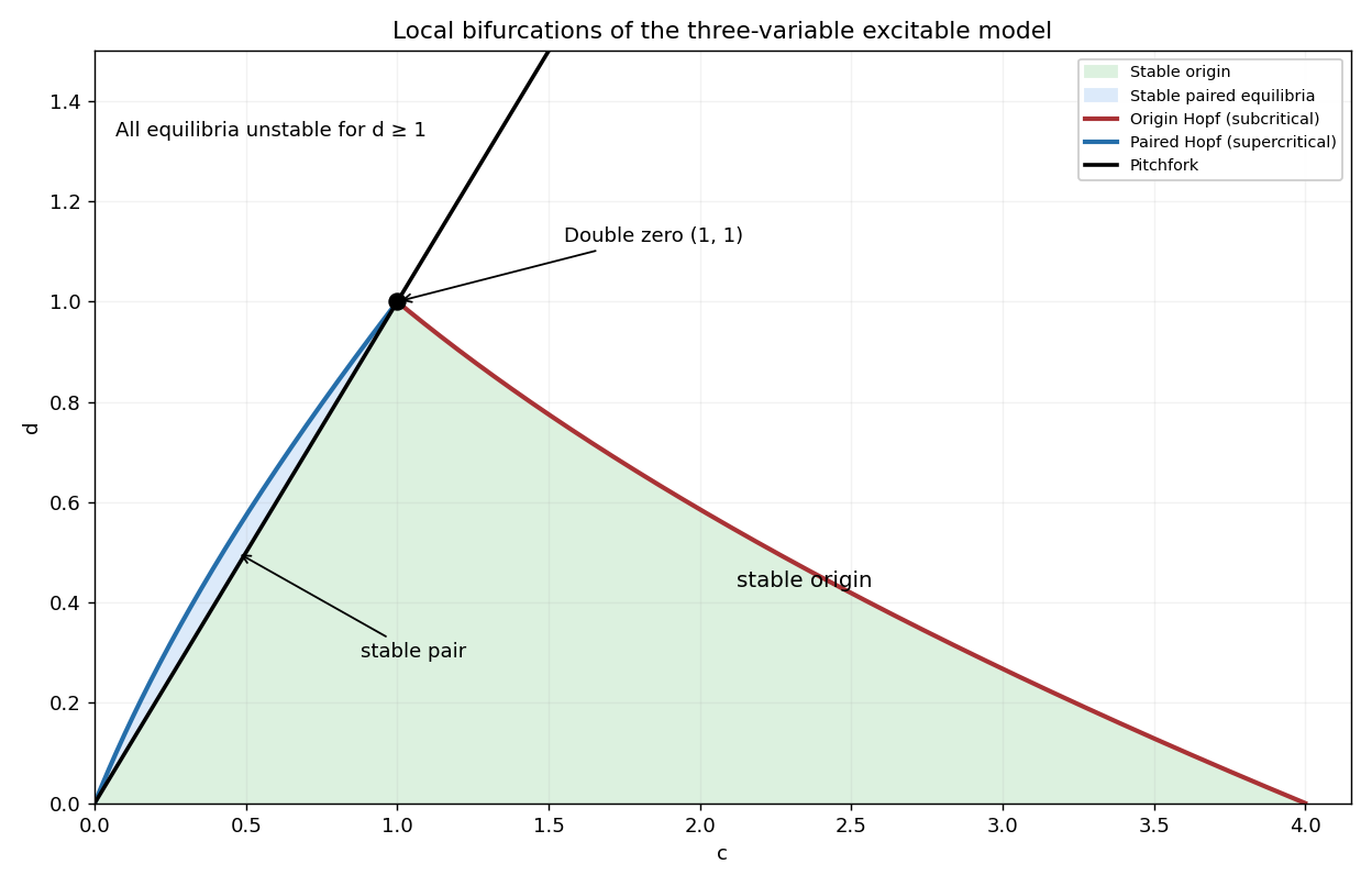
Codex 0 Created 2026-10-03 Updated 2026-10-14A simple zero eigenvalue occurs on , except at . The odd symmetry of the vector field gives a pitchfork bifurcation. Near this curve the critical eigenvalue isFor the other two eigenvalues are stable: this is a supercritical pitchfork bifurcation as decreases through . For it is a subcritical pitchfork bifurcation in the center direction, with an already unstable transverse direction.
For a Hopf bifurcation, factor the characteristic polynomial as . Comparing coefficients givesThus the trivial branch has the local bifurcation curvesThe second curve is a Hopf bifurcation with a stable third eigenvalue. The Routh-Hurwitz stability criterion gives the stable trivial region , . Its Hopf bifurcation is subcritical. To check the sign, normalize the critical right eigenvector by and putThe second component of the normalized left projection is . There is no quadratic term at the origin, and the cubic derivative in the second component is . The cubic Hopf coefficient is therefore . A small repelling periodic orbit lies on the stable-origin side. The diagram also includes the nonzero-branch information derived next.
Past exam of the mathematics course of the University of Cambridge 2001 iii Paper 51 1 b Solution by Codex 0 Created 2026-10-03 Updated 2026-10-14
Codex 0 Created 2026-10-03 Updated 2026-10-14The linearization of this reduction of the FitzHugh-Nagumo model at its trivial equilibrium point isA double zero eigenvalue requires both the constant and linear coefficients to vanish. Hence the codimension-two point isThere the polynomial is . The kernel of a linear map of is one-dimensional, so its zero eigenvalue has a nontrivial size-two block in Jordan normal form. This is a reflection-symmetric double-zero point of Bogdanov–Takens bifurcation type, with one stable direction; the nonlinear coefficients are computed below rather than assumed.
Past exam of the mathematics course of the University of Cambridge 2001 iii Paper 51 1 a Solution by Codex 0 Created 2026-10-03 Updated 2026-10-14
Codex 0 Created 2026-10-03 Updated 2026-10-14Write for the homogeneous cubic correction and for the nilpotent linear part. The chain rule gives the transformed cubic vector field as . Thus the cubic coefficients in the first equation arewhile those in the second equation areConsequently one explicit near-identity transformation isThe transformed equations have no cubic correction in , and only survive in . The cubic coefficients areThis is the cubic elimination at a nilpotent double-zero point; the extra is the nilpotent cubic damping invariant contribution from the first equation. Higher-order terms generated by the substitution are outside the cubic truncation.
Pinned article: Introduction to the OurBigBook Project
Welcome to the OurBigBook Project! Our goal is to create the perfect publishing platform for STEM subjects, and get university-level students to write the best free STEM tutorials ever.
Everyone is welcome to create an account and play with the site: ourbigbook.com/go/register. We belive that students themselves can write amazing tutorials, but teachers are welcome too. You can write about anything you want, it doesn't have to be STEM or even educational. Silly test content is very welcome and you won't be penalized in any way. Just keep it legal!
Intro to OurBigBook
. Source. We have two killer features:
- topics: topics group articles by different users with the same title, e.g. here is the topic for the "Fundamental Theorem of Calculus" ourbigbook.com/go/topic/fundamental-theorem-of-calculusArticles of different users are sorted by upvote within each article page. This feature is a bit like:
- a Wikipedia where each user can have their own version of each article
- a Q&A website like Stack Overflow, where multiple people can give their views on a given topic, and the best ones are sorted by upvote. Except you don't need to wait for someone to ask first, and any topic goes, no matter how narrow or broad
This feature makes it possible for readers to find better explanations of any topic created by other writers. And it allows writers to create an explanation in a place that readers might actually find it.
Figure 1. Screenshot of the "Derivative" topic page. View it live at: ourbigbook.com/go/topic/derivativeVideo 2. OurBigBook Web topics demo. Source. - local editing: you can store all your personal knowledge base content locally in a plaintext markup format that can be edited locally and published either:This way you can be sure that even if OurBigBook.com were to go down one day (which we have no plans to do as it is quite cheap to host!), your content will still be perfectly readable as a static site.
- to OurBigBook.com to get awesome multi-user features like topics and likes
- as HTML files to a static website, which you can host yourself for free on many external providers like GitHub Pages, and remain in full control

Figure 2. You can publish local OurBigBook lightweight markup files to either OurBigBook.com or as a static website.
Figure 3. Visual Studio Code extension installation.
Figure 5. . You can also edit articles on the Web editor without installing anything locally. Video 3. Edit locally and publish demo. Source. This shows editing OurBigBook Markup and publishing it using the Visual Studio Code extension. 
- Infinitely deep tables of contents:




All our software is open source and hosted at: github.com/ourbigbook/ourbigbook
Further documentation can be found at: docs.ourbigbook.com
Feel free to reach our to us for any help or suggestions: docs.ourbigbook.com/#contact