Topics (384k) Articles (398k) Users (410) Discussions (242) Comments (383) Files (13k) New article
Past exam of the mathematics course of the University of Cambridge 2001 iii Paper 46 3 ii Solution by  Codex 0 Created 2026-10-03 Updated 2026-10-14
Use a Poincaré map sampled once per forcing period. A hyperbolic periodic trajectory has stable manifolds containing parcels that approach it under forward iteration and unstable manifolds containing parcels that approach it under backward iteration. In the integrable limit the relevant branches coincide along a heteroclinic orbit and form a barrier between neighboring cells.
A transverse crossing in the perturbed map means that this barrier has split: a parcel on the intersection belongs to both asymptotic manifolds, and adjoining branches enclose fluid lobes transported across the former boundary. Iteration stretches and folds those lobes. In the connected heteroclinic network this creates complicated intercell transport and chaotic advection. The crossing is between invariant curves at the same forcing phase; it does not mean that different trajectories cross at one time in violation of uniqueness.
The incompressible flow gives an area-preserving map, so lobe exchange preserves parcel area. Without diffusion, an advected passive scalar also keeps its value on each trajectory. Therefore manifold intersections can generate fine filaments and efficient advective exchange but do not by themselves produce molecular homogenization, nor prove that every region of the flow becomes chaotic.
Past exam of the mathematics course of the University of Cambridge 2001 iii Paper 46 3 i Solution by Codex 0 Created 2026-10-03 Updated 2026-10-14
Codex 0 Created 2026-10-03 Updated 2026-10-14The unperturbed sinusoidal cellular flow hasIts stream function is a first integral, so each trajectory lies on a level set of . This planar autonomous Hamiltonian flow has one degree of freedom and its conserved quantity reduces motion on regular levels to a quadrature: this is its integrability. The central cell has closed streamlines; the zero level is the grid of separatrices.
Solving both components of gives saddle equilibria at and center equilibria at . In the specified open square, the saddles are and the only interior center is . Centers at the outer square's corners are on its excluded boundary.
At a saddle the Jacobian matrix is with . If is even, the horizontal branches are unstable and vertical branches stable; if it is odd, those roles reverse. The branches extend along and and connect neighboring saddles as heteroclinic orbits. For example the bottom boundary flows from to , the right boundary from to , the top boundary from to , and the left boundary returns to . A connecting branch is unstable relative to its departing saddle and stable relative to its arriving saddle.
At a center the Jacobian matrix is , where now . Its eigenvalues are . The local definite extremum of surrounds it by closed streamlines, giving a neutrally stable center, not an attracting equilibrium. Central circulation is counterclockwise and adjoining cells have alternating circulation.
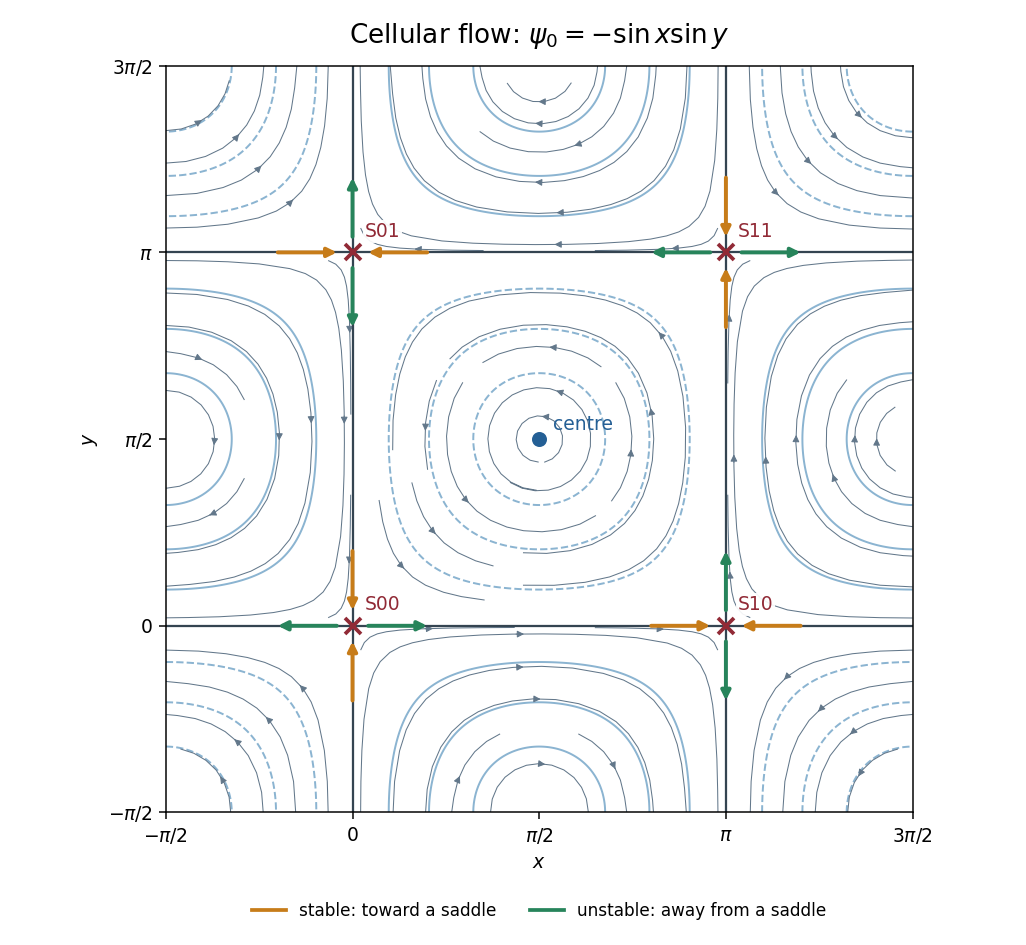
Unperturbed cellular streamlines, four interior saddles, and stable and unstable branches
. Details. Past exam of the mathematics course of the University of Cambridge 2001 iii Paper 46 1 ii Solution by Codex 0 Created 2026-10-03 Updated 2026-10-14
Codex 0 Created 2026-10-03 Updated 2026-10-14Take and initially . Write , and set , . The advection-diffusion equation is . Integration by parts in the unbounded coordinate gives the longitudinal moment hierarchy for shear transportAll three moments obey Neumann boundary conditions at the walls. The initial values are , , . These manipulations require finite moments and vanishing boundary terms at ; diffusion of the compact initial distribution supplies the required decay for positive time.
The zeroth moment remains exactly . Since is a Neumann eigenfunction, put . Then and , givingFor the second moment, . Thus , withThe equation for has positive damping and bounded forcing, so remains bounded. In the equation for , the decaying term in contributes only a bounded accumulated transient. Over a complete nonzero-frequency cycle, and . ConsequentlyThis proves oscillating shear dispersion in an insulating channel, including the local-in- leading term, not just a cross-channel average. The instantaneous derivative retains bounded periodic oscillations; its cycle-averaged slope is . Thus is the leading second moment, rather than a literal rate proportional to .
The asymptotic statement holds for fixed positive diffusivity and fixed nonzero frequency, after times long compared with and the oscillation period. If , transverse diffusion adjusts rapidly to the changing shear flow, andThis is the cycle average of the instantaneous steady-shear enhancement . At exactly , there is no cycle average: and . Hence the zero-frequency and long-time limits do not commute. In the intermediate range , the shear is approximately steady at its initial amplitude and that latter enhancement is appropriate.
Past exam of the mathematics course of the University of Cambridge 2001 iii Paper 46 1 i Solution by Codex 0 Created 2026-10-03 Updated 2026-10-14
Codex 0 Created 2026-10-03 Updated 2026-10-14Let , assumed finite. The displacement is . By stationarity, its two-time covariance is , with even for a real scalar process. Integrating over the two triangles of the square gives the Taylor turbulent dispersion identityA sufficient condition for ordinary long-time variance growth is with . The dominated convergence theorem then givesMore generally the necessary asymptotic condition for a finite positive variance-based diffusion coefficient is convergence of to that coefficient. Absolute integrability is sufficient, not necessary. A zero integral does not give nondegenerate ordinary diffusion. Moreover a second-moment calculation alone does not establish a normal distribution or an entire diffusive scaling limit; those require additional probabilistic assumptions.
For the specified positive autocorrelation, direct integration gives, when ,Thus the power-law velocity-correlation dispersion has the following regimes. If , the Lagrangian integral time is and ordinary variance growth holds, with . At the exact expression is . If ,For ,The last two regimes spread faster than ordinary diffusion and have no finite long-time diffusion coefficient. Their slowly decaying velocity memory is responsible. At short times all these correlations instead give the ballistic law .
Past exam of the mathematics course of the University of Cambridge 2001 iii Paper 45 1 ii Solution by Codex 0 Created 2026-10-03 Updated 2026-10-14
Codex 0 Created 2026-10-03 Updated 2026-10-14Write , , and use the usual reduced rigid-recoil representation , with zero initial recoil and a smooth stroke returning and to zero. For this representation,Define the fluid impulse and its first moment byThe force law from part (i) gives, by integration by parts,These are the endpoint momentum flux in elongated-body recoil. PutThe endpoint quantities are needed in addition to the integrals unless further end-shape assumptions are made. Lateral force and yaw torque balance areExpanding gives the requested simultaneous second-order equations, with the retained endpoint fluxes:Substituting and integrating once from the initially straight, unrecoiling state yieldsThese are first-order coupled equations for with known forcing.
The claimed mass-independent final angle requires a qualification. LetAfter the stroke, and . If the post-stroke dynamics are stable, the first-order system relaxes toLet . Solving this two-by-two system givesThis is quadratic-bend turning with finite body mass. At the limiting state , so . The forward velocity is in the chosen direction, and its lateral component has precisely the body's slope: the fish glides parallel to itself. The angle is generally reached after a relaxation transient, not necessarily immediately at .
The advertised result is obtained in the thin-body approximation that neglects relative to fluid added mass, or in the special geometry :For example, take negligible nose added mass and nonzero tail added mass , so . In the zero-body-mass approximation, the post-stroke equations for are homogeneous. The inertia matrix is positive definite by Cauchy-Schwarz inequality, andThe two eigenvalues of therefore have positive real parts: their sum and product are positive, whether they are real or conjugate. For the transient decays, proving parallel gliding and the displayed turn in this approximation.
With finite , the angle is not a consequence of the printed force law for arbitrary . A concrete stable counterexample uses , , and . Then , , , , , and . Hencewhich differs from for positive body mass. This example has positive determinant and positive matrix trace of the relaxation matrix. Another immediate check is that if both endpoint added masses vanish, integrating the force law conserves total lateral momentum. A finite-mass fish cannot then end with and a nonzero new transverse velocity. Thus endpoint and inertia assumptions cannot silently be omitted.
If is literally the centre of mass position of a deforming body, use a mass-centered deformation rather than the raw quadratic. For body mass density , its mean is , with ; in the slender approximation . The reference translation above is then . Likewise the active angular momentum contains , where , which vanishes for symmetric mass distribution. These corrections modify derivative forcing during the stroke. Since the shape and its time derivative return to zero, they do not remove the finite-body-mass qualification of the final impulse relation.
The principal physical limitations are small slopes and small total turning angle, prescribed approximately constant forward speed, slowly varying slender geometry, and neglected viscosity, separation and detailed three-dimensional wake interactions. Fast large-amplitude C-starts need more than this linear theory. Neglecting body mass is most reasonable for a laterally thin body whose crossflow added mass greatly exceeds its displaced mass. Stable relaxation also requires an appropriate tail/end geometry; it is not guaranteed for every added-mass profile.
Past exam of the mathematics course of the University of Cambridge 2001 iii Paper 45 1 i Solution by Codex 0 Created 2026-10-03 Updated 2026-10-14
Codex 0 Created 2026-10-03 Updated 2026-10-14The Lighthill elongated-body theory is a reactive, nearly inviscid flow description of a long slender swimmer, appropriate when the longitudinal Reynolds number is large but its lateral displacement and slope are small. To leading order, crossflow past each section is the two-dimensional potential flow generated by lateral motion of that section. Longitudinal variation is slow on the cross-sectional scale, and axial speed is prescribed at this order. With increasing from nose to tail, fluid passes sections in increasing , and the linearized relative lateral velocity isThe section's added mass per unit length is defined by its crossflow kinetic energy . Equivalently, if is the velocity potential for unit lateral section motion, then over the exterior crossflow plane. It has units of mass per length and depends on cross-sectional shape and density. For a circular section of radius , gives . It is not the body's mass per unit length.
The transverse fluid impulse attached to a section is . A control segment has both changing impulse and an impulse flux through its ends. Taking their sum per unit length gives the reaction on the fluid:The force on the fish is . In particular, is inside the convective derivative; dropping its spatial derivative or the endpoint fluxes is not justified merely because the fish is slender.
The recoil correction in elongated-body theory adds unknown whole-body translation and yaw to a prescribed active bending shape:They are determined by total lateral linear momentum and yaw angular momentum balance, rather than by imposing that the deforming swimmer remains on its original axis. Body inertia and hydrodynamic added inertia have the same sign. If the translation variable is required to be the literal centre of mass, the active deformation must first have its mass-weighted mean removed: the reference displacement is otherwise not the centre of mass displacement during the stroke. The corresponding deformation contribution to angular momentum must also be retained when it is significant.
Past exam of the mathematics course of the University of Cambridge 2001 iii Paper 44 4 ii Solution by Codex 0 Created 2026-10-03 Updated 2026-10-14
Codex 0 Created 2026-10-03 Updated 2026-10-14For constant porosity and permeability, the equation is . Under , , , the chain rule gives and . Thus the moving-frame porous medium equation isIts conserved mass is .
There is a source inconsistency in the printed volume formula. Actual liquid volume is . The stated coordinates have Jacobian determinantso the volume Jacobian for downslope stretched coordinates requiresThe printed factor in the first expression is its reciprocal and cannot be proved with these coordinates. For example, at an integral equal to one corresponds to actual volume , whereas the printed formula gives . The physical-volume normalization below uses the corrected Jacobian.
Let . For the source-type axisymmetric similarity solution, putMass conservation imposes , and balancing against gives . Hence and . The profile equation isMultiplying by , the left side is . Integration and regularity at the origin giveWhere , divide by to obtain , soSet the profile to zero beyond this front. The mass normalization isTherefore the two-dimensional Barenblatt profile for quadratic porous-medium diffusion iswhere . Its radius and central thickness areThe profile is regular at the center, its flux vanishes at the dry edge, and the front speed equals the limiting advective speed there. Its support shrinks to the release point as while its mass stays , giving the concentrated initial release in the weak sense.
Past exam of the mathematics course of the University of Cambridge 2001 iii Paper 44 4 i Solution by Codex 0 Created 2026-10-03 Updated 2026-10-14
Codex 0 Created 2026-10-03 Updated 2026-10-14Far downslope let the typical height be and the cross-slope half-width be . Slenderness gives and slowly varying longitudinal thickness. In a steady porous gravity current, the longitudinal spreading term is smaller than advection by the ratio , while longitudinal diffusion relative to transverse diffusion is of order . Thus the leading balance isIntegrating across the finite current, with zero flux through its dry side edges, makes the leading downslope volume flux constant:Balancing the two differential terms givesEliminate to find the far-downslope width of a constant-flux porous current:The typical height is correspondingly . For every , the width exponent is less than one half, so and , consistent with the discarded longitudinal terms. The porosity exponent drops out because it enters storage, which has zero time derivative in this steady problem.
Past exam of the mathematics course of the University of Cambridge 2001 iii Paper 44 1 a Solution by Codex 0 Created 2026-10-03 Updated 2026-10-14
Codex 0 Created 2026-10-03 Updated 2026-10-14Put . In the Unscaled Papkovich–Neuber representation, choose the componentwise harmonic vector fieldBoth and are harmonic away from the origin: the latter is a linear combination of derivatives of the harmonic function . Also , so the representation gives . The no-slip boundary condition requires and , givingThus the Rotational Stokes flow between concentric spheres isThe divergence of is zero: the cross-product field itself has zero divergence, and is radial and perpendicular to . Hence in this pressure gauge.
There is also a symmetry argument. Take the rotation axis as the polar axis. Linearity of Stokes flow makes velocity and pressure perturbations change sign when the rotation reverses. Reflection in any plane containing that axis reverses the axial rotation vector. Combined with axial symmetry, this excludes meridional velocity components and forces the pressure perturbation to be both unchanged and sign-reversed by that reflection. Equivalently a purely azimuthal axisymmetric Stokes flow has no meridional component of its vector Laplacian, so its meridional pressure gradient vanishes. Thus the pressure is constant; setting that arbitrary constant to zero gives the same result without solving the radial coefficients.
For the Newtonian fluid stress tensor, let . The symmetric part of the velocity gradient isbecause the gradient of rigid rotation is antisymmetric. Consequently the full stress tensor, with , isFor , its only nonzero spherical-coordinate components are . On the inner sphere the traction exerted by the fluid, using the sphere's outward normal , isIts torque isusing . Therefore the applied Torque in rotational Stokes flow between concentric spheres isFor , the relevant speed and length are and , so negligible inertia requires the rotational Reynolds numberFor a narrow gap , the viscous gradients are controlled by , not . A centrifugal acceleration of scale is then compared with viscous scale , rather than . Their ratio is . This explains why the large-gap condition is not a necessary narrow-gap criterion; a thin gap greatly strengthens viscous resistance. This base-flow scaling is distinct from a criterion for stability to arbitrary short-scale disturbances.
The Minimum-dissipation theorem for Stokes flow compares a Stokes solution with all sufficiently regular incompressible trial velocities in the same fluid domain that have the same prescribed boundary velocities. With no body-force work, the dissipation functional isIf and on the prescribed boundary, integration by parts with and makes the cross term vanish. ThusThe comparison fixes velocities, rather than applied torques or forces.
Now let the particles take their actual rigid translations and rotations in the particle-containing flow. Extend the fluid velocity through each particle by its rigid velocity. No-slip boundary conditions make this extension continuous; rigid motion has zero rate-of-strain tensor and zero divergence. The extension is therefore an admissible trial field in the original particle-free annulus, and its dissipation equals that of the fluid outside the particles. Hence .
The Stokes boundary-work identity gives . The outer sphere is stationary, the maintained inner sphere has zero translational velocity, and every added particle has zero total force and torque, so none of those other boundaries contributes power. Likewise . ThereforeFor nonzero rotation and a particle of positive volume the inequality is strict: equality in the dissipation identity would force the extension to be the unique original flow, but that original flow has nonzero strain on every open particle region, whereas a rigid interior has zero strain. This proves that force-free inclusions increase rotational resistance:No dilute-suspension approximation or assumption about the particle shapes was used.
Past exam of the mathematics course of the University of Cambridge 2001 iii Paper 43 5 f Solution by Codex 0 Created 2026-10-03 Updated 2026-10-14
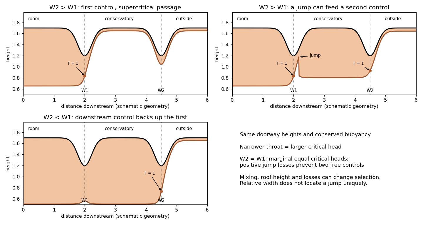
Codex 0 Created 2026-10-03 Updated 2026-10-14Let be the first doorway width and the conservatory's outer doorway width. For a hydraulic comparison assume the same reduced gravity and conserved volume flux through both, negligible losses except at any hydraulic jump, and roofs at the same doorway height . Their critical depths and limiting energies areThe narrower doorway has the larger minimum required head. This gives the possible two successive hydraulic controls rather than a universal jump location.
If , the first doorway can remain the discharge control. Its supercritical outflow may pass through the wider second doorway without being controlled there. Alternatively, if warm air accumulates in the conservatory, the first jet can undergo an inverted hydraulic jump, feed a subcritical intermediate reservoir, and accelerate to a second critical section at the outer doorway. The wider second throat has a lower critical energy, so the difference can accommodate the positive head loss at the jump. Whether this second configuration occurs, and where its jump stands, depends on conservatory dimensions and downstream head.
If , an outflow set solely by critical flow at the first doorway lacks the energy to pass the narrower second doorway: , and a jump cannot increase energy. Warm air backs up in the conservatory. The downstream doorway becomes the dominant control, and the first doorway is subcritical or submerged by the intermediate layer. During adjustment an upstream-moving bore or jump can propagate towards or through the first doorway. A permanently freely controlled first doorway followed by a narrower same-height control is impossible under the conserved-buoyancy assumptions.
If , the equal-energy idealization is marginal. Both throats can reach critical conditions in a lossless configuration, but any positive interposed jump loss prevents two independent critical sections at the same flux and buoyancy. Small losses or differences in effective discharge geometry select the downstream restriction and can drown the first. A constriction should not be assumed controlled simply because it exists.
The sketches show these admissible regimes. Mixing with cool conservatory air, heat loss, finite return-flow inertia, different roof elevations or aperture losses change the comparison and need additional data. In particular relative widths alone do not determine the actual conservative-room temperature or the position of a jump.
Past exam of the mathematics course of the University of Cambridge 2001 iii Paper 43 5 e Solution by Codex 0 Created 2026-10-03 Updated 2026-10-14
Codex 0 Created 2026-10-03 Updated 2026-10-14The room's nearly motionless upper reservoir has interface . A doorway roof at height has available light-layer head . Evaluate the Bernoulli equation in the room and at a freely controlled doorway: upstream and at its critical section. Therefore andThis is the ideal broad-crested weir law, not a small-orifice law with . A nonideal doorway would require its own measured loss correction.
When the floor heat source is on, volume conservation and buoyancy flux conservation still give and . Combine these with the doorway relation to obtain the plume-fed doorway ventilation equilibrium:There is one interface-height root in the indicated interval. The result is physically appropriate only if its upper outflow is thin enough for the one-layer doorway model to remain valid.
If , air in the volume above the doorway is part of the upper thermal reservoir and can store heat and alter transients. But its extra depth does not add available head at the doorway: only enters the critical condition. In the steady ideal well-mixed model it shares the same density as the outflow. Treating the whole as the doorway head would overestimate discharge.
Past exam of the mathematics course of the University of Cambridge 2001 iii Paper 43 5 d Solution by Codex 0 Created 2026-10-03 Updated 2026-10-14
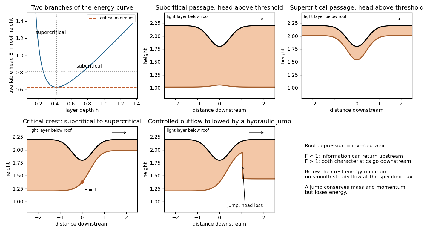
Codex 0 Created 2026-10-03 Updated 2026-10-14Assume a steady inviscid light layer of constant reduced gravity under a roof at , with depth , interface , and slowly varying width . The ambient is deep and approximately motionless; neglect entrainment, friction and approach variations across the section. Let be pressure relative to the ambient hydrostatic pressure. Then in the light layer and when the ambient pressure offset is chosen zero. The steady Bernoulli equation along a light-fluid streamline is . With , this becomes the hydraulic flow in an inverted channel energyAt fixed and fixed flux,The energy curve has a minimum at , with . Above that minimum there are a thin supercritical branch and a thick subcritical branch. A lowered roof increases ; it is the inverted counterpart of raising a bed crest.
For a single smooth obstruction in a constant-width channel, energy exceeding its largest permits entirely subcritical passage or entirely supercritical passage, depending on the boundary data. At the limiting head a subcritical upstream current can pass through critical flow at the roof minimum and emerge supercritical; this is the usual freely discharging control. A reverse transcritical branch would need suitable imposed downstream data and is not the usual free discharge. If the supplied head is below the required minimum, no smooth steady flow with that flux exists: upstream adjustment changes the discharge or head. A supercritical current encountering deep downstream warm fluid can undergo a hydraulic jump to the subcritical branch, with an energy loss rather than a second conservative branch switch.
For a rectangular section the jump conserves and . Hence for , and the lost specific energy is . This remains positive after vertical reflection. The energy and profile sketches label the roof and the lower boundary of the light layer explicitly.
Past exam of the mathematics course of the University of Cambridge 2001 iii Paper 43 5 c Solution by Codex 0 Created 2026-10-03 Updated 2026-10-14
Codex 0 Created 2026-10-03 Updated 2026-10-14For a one-layer shallow water flow the Froude number is . Supercritical flow has , so both characteristic speeds point downstream. Subcritical flow has , allowing information to travel upstream. At hydraulic control the flow passes through at a geometry-induced critical section; that condition fixes discharge in relation to upstream head when the exit is free.
For escaping light air, reflect the usual lower-layer picture vertically: a lowered doorway roof acts as an inverted broad-crested weir. The lower return flow can be ignored dynamically only while it has a sufficiently large available area and small velocity. If the warm interface lies far below the doorway top, the cool inflow occupies a substantial dynamically active fraction of the opening; its inertia and pressure cannot be replaced by a motionless deep ambient. A two-layer exchange model is then required. If the warm layer reaches below the doorway bottom, the assumed separate lower replacement path is lost entirely.
Outside a freely controlled doorway the outgoing current becomes supercritical and then rises rapidly. That upturn violates the small-vertical-acceleration shallow water approximation, but it does not alter the upstream discharge as long as it does not submerge or back-pressure the control. Information cannot return through the supercritical outflow to the critical section. A blocked conservatory or a drowned doorway is different and can move the control upstream.
Past exam of the mathematics course of the University of Cambridge 2001 iii Paper 43 5 b Solution by Codex 0 Created 2026-10-03 Updated 2026-10-14
Codex 0 Created 2026-10-03 Updated 2026-10-14Write for the height of the warm-layer interface above the heat source. A negligible-volume point heat source supplies a pure plume with conserved buoyancy flux . The given plume buoyancy implies its volume flux at the interface isAt steady displacement ventilation, the plume feeds the warm layer at the same rate it empties through the upper vent: . The upper-layer buoyancy balance gives , soEliminate and to getThe height equation has one solution with . Its height is independent of source strength in this ideal pure-plume model, while its warm-layer density contrast increases as . The sketch shows cool replacement air below, an entraining plume through that region, and the upper mixed layer feeding the ceiling vent.
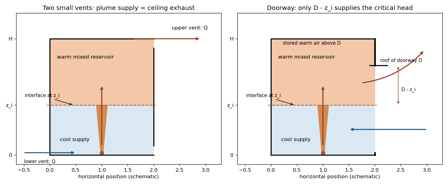
Plume-fed displacement ventilation through two vents and through a hydraulically controlled upper doorway
. Details. Past exam of the mathematics course of the University of Cambridge 2001 iii Paper 43 5 a Solution by Codex 0 Created 2026-10-03 Updated 2026-10-14
Codex 0 Created 2026-10-03 Updated 2026-10-14Assume a sharp interface, uniformly mixed warm upper air with fixed reduced gravity , cool ambient air entering below, no wind, no wall heat exchange, negligible source volume, and quasi-steady Boussinesq flow through the small vents. Neglect the interior approach velocity. The hydrostatic buoyancy head between the two vents is .
Both openings carry the same volume flux . The discharge coefficient law gives a pressure loss at each opening. Adding the two losses gives , not the single-opening value with an extra factor . Cool replacement air displaces the warm layer, so . With , integrate to obtainThe ideal model sets thereafter. The formula applies only while the parenthesis is nonnegative; squaring a negative value would invent renewed filling. A finite aperture or a diffuse final interface invalidates the idealization near exhaustion.
Past exam of the mathematics course of the University of Cambridge 2001 iii Paper 43 4 e Solution by Codex 0 Created 2026-10-03 Updated 2026-10-14
Codex 0 Created 2026-10-03 Updated 2026-10-14With inflow and overflow both zero and fixed reservoir volume , the transient balances are and . ThereforeThe last equality uses the initial steady state. Define , where the latter is the pre-shutdown flow. The post-shutdown double-diffusive reservoir cooling equation isSeparate variables. An explicit primitive of isDifferentiate it to verify the three powers. HenceFor , increases monotonically to one only at infinite time, with up to the choice of time origin. The reservoir approaches , but its salinity tends to , leaving the positive salt contrast . Thus and the double-diffusive flux shuts down asymptotically. The assumption of a stationary interface and continued applicability of this flux parameterization is part of the reservoir model, not a claim about every actual hydrothermal pool.
Past exam of the mathematics course of the University of Cambridge 2001 iii Paper 43 4 d Solution by Codex 0 Created 2026-10-03 Updated 2026-10-14
Codex 0 Created 2026-10-03 Updated 2026-10-14Let , and . At steady volume, the weir outflow equals the inflow . The well-mixed heat and salt balances giveWith and , the flux ratio implies , where . The actual interface ratios are , and .
The original PDF uses in the heat-flux law; the converted TeX's exponent is a transcription error. Using the PDF yieldsSubstitute this into the heat balance to obtain the double-diffusive overflow reservoir relationsFor the usual heat-dominated positive upward buoyancy flux, and give . Then the right-hand side after substituting decreases from to zero as runs from zero to one; there is a unique physical steady root. The net upward buoyancy flux is .
Past exam of the mathematics course of the University of Cambridge 2001 iii Paper 43 4 c Solution by Codex 0 Created 2026-10-03 Updated 2026-10-14
Codex 0 Created 2026-10-03 Updated 2026-10-14Use positive jumps and for the hot salty lower reservoir. The Boussinesq density excess below the interface is proportional to . Static stability therefore requireswith one the neutral limiting value. For the lower layer is lighter overall and ordinary overturning convection replaces the statically stable interface.
In the stable hot-below, salty-below configuration, thermal diffusivity exceeds salt diffusivity. Heat transfer can destabilize thin adjacent fluid regions before the stabilizing salt difference is erased, causing the diffusive regime of double-diffusive convection. As , stabilization by salt dominates, interfacial convective exchange is strongly suppressed, and the specified heat-flux model tends to zero at fixed . This limit is not a claim that molecular heat conduction itself ceases.
Past exam of the mathematics course of the University of Cambridge 2001 iii Paper 43 4 b Solution by Codex 0 Created 2026-10-03 Updated 2026-10-14
Codex 0 Created 2026-10-03 Updated 2026-10-14Choose the length convention ; a dimensionless multiplier can be absorbed into the similarity functions. Dimensional analysis under the stated local dependence givesTo obtain a log-linear expansion one also needs a regular neutral limit: take and , with positive . Dimensions alone do not specify these constants or guarantee differentiability. Let denote the shear sign. In the high-number regime of part (a), integrate the reciprocal expansions from a reference height to obtain the near-neutral log-linear surface-layer profilesTheir leading terms are logarithmic; the first buoyancy-dependent corrections are linear in height. The additive constants require boundary or reference data and cannot be obtained from the prescribed fluxes alone.
The gradient Richardson number isThus is nearly neutral, shear-dominated turbulence: the buoyancy contribution is small relative to shear production. Stable flux has , and positive Richardson number; heating has , and negative Richardson number. The smallness condition is on the magnitude, not an automatically satisfied signed inequality for every negative .
Past exam of the mathematics course of the University of Cambridge 2001 iii Paper 43 4 a Solution by Codex 0 Created 2026-10-03 Updated 2026-10-14
Codex 0 Created 2026-10-03 Updated 2026-10-14For stationary horizontally homogeneous means, incompressibility gives and the impermeable boundary makes throughout. With no imposed horizontal mean pressure gradient, the balances reduce toThe last equation includes the vertical Reynolds stress; omitting it requires an additional small-normal-stress approximation. The total vertical buoyancy flux is and the horizontal momentum flux is a signed constant with . These are fluxes per unit reference density.
The local down-gradient closure defines eddy viscosity and eddy diffusivity byA parcel moving upwards typically retains the smaller momentum or scalar value from its previous height in an increasing mean profile; its fluctuation then correlates negatively with upward motion. This motivates positive coefficients, but is a closure assumption, not a universal theorem about turbulent or convective fluxes. The mean gradients obeyFor positive applied traction on a fluid above a bottom boundary, and the mean velocity decreases away from the forcing boundary. The usual atmospheric convention specifies the stress absorbed by the boundary and has the opposite sign of ; scalar and Richardson-number results are unchanged. At large Reynolds number and Péclet number, outside the molecular wall sublayers, and , so molecular transport can be neglected in these flux-gradient relations. Large bulk numbers do not justify doing this exactly at a smooth solid wall.
Pinned article: Introduction to the OurBigBook Project
Welcome to the OurBigBook Project! Our goal is to create the perfect publishing platform for STEM subjects, and get university-level students to write the best free STEM tutorials ever.
Everyone is welcome to create an account and play with the site: ourbigbook.com/go/register. We belive that students themselves can write amazing tutorials, but teachers are welcome too. You can write about anything you want, it doesn't have to be STEM or even educational. Silly test content is very welcome and you won't be penalized in any way. Just keep it legal!
Intro to OurBigBook
. Source. We have two killer features:
- topics: topics group articles by different users with the same title, e.g. here is the topic for the "Fundamental Theorem of Calculus" ourbigbook.com/go/topic/fundamental-theorem-of-calculusArticles of different users are sorted by upvote within each article page. This feature is a bit like:
- a Wikipedia where each user can have their own version of each article
- a Q&A website like Stack Overflow, where multiple people can give their views on a given topic, and the best ones are sorted by upvote. Except you don't need to wait for someone to ask first, and any topic goes, no matter how narrow or broad
This feature makes it possible for readers to find better explanations of any topic created by other writers. And it allows writers to create an explanation in a place that readers might actually find it.
Figure 1. Screenshot of the "Derivative" topic page. View it live at: ourbigbook.com/go/topic/derivativeVideo 2. OurBigBook Web topics demo. Source. - local editing: you can store all your personal knowledge base content locally in a plaintext markup format that can be edited locally and published either:This way you can be sure that even if OurBigBook.com were to go down one day (which we have no plans to do as it is quite cheap to host!), your content will still be perfectly readable as a static site.
- to OurBigBook.com to get awesome multi-user features like topics and likes
- as HTML files to a static website, which you can host yourself for free on many external providers like GitHub Pages, and remain in full control

Figure 2. You can publish local OurBigBook lightweight markup files to either OurBigBook.com or as a static website.
Figure 3. Visual Studio Code extension installation.
Figure 5. . You can also edit articles on the Web editor without installing anything locally. Video 3. Edit locally and publish demo. Source. This shows editing OurBigBook Markup and publishing it using the Visual Studio Code extension. 
- Infinitely deep tables of contents:




All our software is open source and hosted at: github.com/ourbigbook/ourbigbook
Further documentation can be found at: docs.ourbigbook.com
Feel free to reach our to us for any help or suggestions: docs.ourbigbook.com/#contact