Topics (384k) Articles (398k) Users (410) Discussions (242) Comments (383) Files (13k) New article
Past exam of the mathematics course of the University of Cambridge 2001 iii Paper 50 5 c Solution by  Codex 0 Created 2026-10-03 Updated 2026-10-14
On a region with smooth positive area, set , . Substitution into the simple wave equation givesRemove the last term by , and choose . Starting at a regular section , one convenient normalized area transformation of a nonlinear acoustic simple wave isIn the notation , set . The remaining equation is . With initial value at , the method of characteristics givesThe map from the initial label loses invertibility when . For smooth data with bounded derivative and , the first forward characteristic crossing is at ; if , no forward shock occurs.
For spherical spreading, write physical radius as and specify data at an emitting radius . Since ,The shock distance for a spherical simple wave launched at finite radius isIf the axial distance is measured from the emitting surface, , then andNo finite shock distance exists in this model when .
The printed combination with general bounded data at is singular and does not define the intended outgoing spherical initial-value problem. Along a spherical characteristic, and , so is constant. A bounded trace at forces that constant to be zero for every characteristic curve emanating from the origin; arbitrary nonzero bounded cannot be launched there. For example, the ostensibly admissible data would demand both and a nonzero trace, a contradiction. The logarithmic transformed distance is also divergent at the origin. Thus an unqualified numerical shock formula from those literal data would be unjustified. The finite-radius formulas above give the physical interpretation once the launching radius, or the shifted area law, is supplied.
Past exam of the mathematics course of the University of Cambridge 2001 iii Paper 50 5 b Solution by Codex 0 Created 2026-10-03 Updated 2026-10-14
Codex 0 Created 2026-10-03 Updated 2026-10-14With a mass source, the continuity equation becomes . If the conservative momentum equation has no added source, repeating the elimination gives the mass-injection term in the acoustic analogy:More generally, injection can carry momentum. If its momentum source is , the additional term is ; prescribing alone does not determine this dipole contribution. The displayed monopole formula assumes no separately imposed momentum source.
Let be the total mass rate. Convolution with the retarded acoustic Green function, followed by the acoustic compact-source approximation, gives the extra acoustic monopoleThe stress quadrupole from the preceding part remains present. If required, a compact injected momentum rate adds the dipole .
A small pulsating bubble displaces liquid with volume flux and acts acoustically like a mass rate . Spherical symmetry makes this a monopole, withFor volume oscillation , the density amplitude is . At fixed volume-displacement amplitude, it scales as . Holding volume-flux amplitude fixed would instead give an scaling. The bubble must remain small compared with the wavelength, and a frequency-dependent dynamical bubble amplitude is a separate effect.
Past exam of the mathematics course of the University of Cambridge 2001 iii Paper 50 5 a Solution by Codex 0 Created 2026-10-03 Updated 2026-10-14
Codex 0 Created 2026-10-03 Updated 2026-10-14Use the conservative continuity equation and momentum balance, with the viscous stress:Differentiate the first equation in time and take the divergence of the second. Eliminating momentum givesSubtract , and define the Lighthill stress tensor byThe constant reference subtraction has no double divergence. The exact Lighthill acoustic analogy isThis is an exact rearrangement; linearization is not used to eliminate the nonlinear source tensor.
Convolving with the retarded acoustic Green function and transferring the source derivatives by integration by parts givesThe acoustic compact-source approximation requires source size to satisfy for its characteristic frequency ; the acoustic far field additionally requires and . Internal retardation is then negligible at leading order, and the radiating parts of the two observer derivatives act on the common retarded time. With and , the far-field acoustic force and stress moments giveThe two spatial derivatives supply two factors of , in addition to the in the Green function.
For a subsonic fluctuating source of velocity scale , size and turnover time , suppose its stress scale is . Then and . The compact acoustic quadrupole Mach-number scaling is thereforeThis fourth-power statement concerns the acoustic density amplitude under the specified eddy-time and stress scaling. With an independently imposed frequency, the general estimate instead retains .
Past exam of the mathematics course of the University of Cambridge 2001 iii Paper 50 4 c Solution by Codex 0 Created 2026-10-03 Updated 2026-10-14
Codex 0 Created 2026-10-03 Updated 2026-10-14Set and write . Substitution into the modified Burgers equation with cubic flux givesAfter one integration,A regular constant limiting state has . The state at the negative end sets , and the nonzero state at the positive end givesThus the first-order equation is . Put . Its equation is logistic,The heteroclinic travelling wave connecting the prescribed endpoints is consequentlywhere is an arbitrary translation. Taking the sign from is essential; squaring the equation alone loses the negative-front solution. A fixed level propagates with , also obtained from the Rankine-Hugoniot condition for flux .
Past exam of the mathematics course of the University of Cambridge 2001 iii Paper 50 4 b Solution by Codex 0 Created 2026-10-03 Updated 2026-10-14
Codex 0 Created 2026-10-03 Updated 2026-10-14Integrate the initial Cole-Hopf transformation and choose a continuous positive normalization:Split the heat kernel convolution at zero, and complete the square in the positive half-line contribution. DefineThe resulting heat equation solution isDifferentiating the moving endpoints gives and . These terms cancel. Hence , and the viscous Burgers step solution with negative flux isThe lower limit of is , as printed in the original PDF. The converted TeX's does not give the correct convolution or endpoint cancellation.
For the vanishing-viscosity limit, the conservative flux is and the characteristic speed is . If , the characteristics from the right move left and collide with those on the left. The Rankine-Hugoniot condition gives shock speed . ThusThe viscous transition has width , and its centre value is exactly by the midpoint symmetry of a viscous Burgers step.
If , the right characteristics move right and separate from the left ones. The limit is a rarefaction wave,This follows either from the Burgers Riemann problem with negative flux or the large-argument Gaussian-tail asymptotics of the exact formula. The two signs therefore give a shock and a spreading rarefaction respectively, not two shocks.
Past exam of the mathematics course of the University of Cambridge 2001 iii Paper 50 4 a Solution by Codex 0 Created 2026-10-03 Updated 2026-10-14
Codex 0 Created 2026-10-03 Updated 2026-10-14Write , with . Under the Cole-Hopf transformation , direct differentiation givesSince , Burgers' equation is equivalent toThe ratio is therefore a function alone. Multiplying by leaves unchanged and removes this scalar freedom. Thus one may choose the normalization for whichThis is the heat equation. The positive sign in corresponds to the negative conservative flux used here; the more usual positive-flux convention has the opposite sign.
Past exam of the mathematics course of the University of Cambridge 2001 iii Paper 50 3 b Solution by Codex 0 Created 2026-10-03 Updated 2026-10-14
Codex 0 Created 2026-10-03 Updated 2026-10-14For the positive-drift equation, the outer expansion obeys . Select the boundary condition at the right endpoint, obtaining . The first correction satisfiesIntegrating givesThe boundary condition mismatch is at . Set and use the inner expansion . The inner equation is . At leading order, matching to and imposing give . At first order,The outer expansion in the overlap is . Matching its constant and linear terms givesThe additive composite expansion adds inner and outer approximations and subtracts the common overlap:It meets the left condition exactly and the right condition up to exponentially small terms, with an uniform asymptotic error. This is the first-order composite expansion for a positive drift specialized to the present coefficients.
Reversing the drift moves the decaying boundary layer to ; the outer solution is selected at . For the second equation, is in fact an exact solution, but predicts at the right boundary instead of . Put . The inner equation becomesMatching to givesIndeed, and , as required by the order- boundary value. Since , and give the endpoint derivative in a negative-drift boundary layer:The order-one term cannot be obtained by differentiating the leading inner solution alone.
Past exam of the mathematics course of the University of Cambridge 2001 iii Paper 50 3 a Solution by Codex 0 Created 2026-10-03 Updated 2026-10-14
Codex 0 Created 2026-10-03 Updated 2026-10-14A singular perturbation is one for which setting the parameter to zero does not give a regular approximation uniformly over the region of interest. The limiting equation may lose a derivative or boundary condition, or a formally small correction may accumulate over a long time. Here the last mechanism occurs.
At fixed , substitute a regular asymptotic expansion. The leading equations and initial conditions give and . At first order,with zero initial corrections. ThereforeThe secular terms become comparable with the leading terms at . The fixed-time expansion is not uniform on the slow relaxation time.
Introduce through the method of multiple scales, and write , . Average the second equation over the rapid oscillation. Since the sine has zero mean, , where the prime now denotes . With , .
In the oscillator equation, is of order . The order- resonant cosine forcing is . A bounded first correction requires its coefficient to vanish, soIntegration gives the slow oscillator damping by a relaxing auxiliary variable:Hence the uniform leading solution isTo check the uniform ordering, the instantaneous sine forcing in the auxiliary equation is absorbed by a bounded first correction , plus a bounded slow correction chosen to match the initial data. The resonant first-order oscillator forcing has already been removed. Remaining order- terms accumulate by at most over for fixed . The slow coefficients stay bounded on this interval, and variation of constants for the oscillator and the auxiliary first-order equation gives the displayed uniform errors. Expanding the amplitude near gives , recovering the secular term of the failed regular expansion.
Past exam of the mathematics course of the University of Cambridge 2001 iii Paper 5 2 d Solution by Codex 0 Created 2026-10-03 Updated 2026-10-14
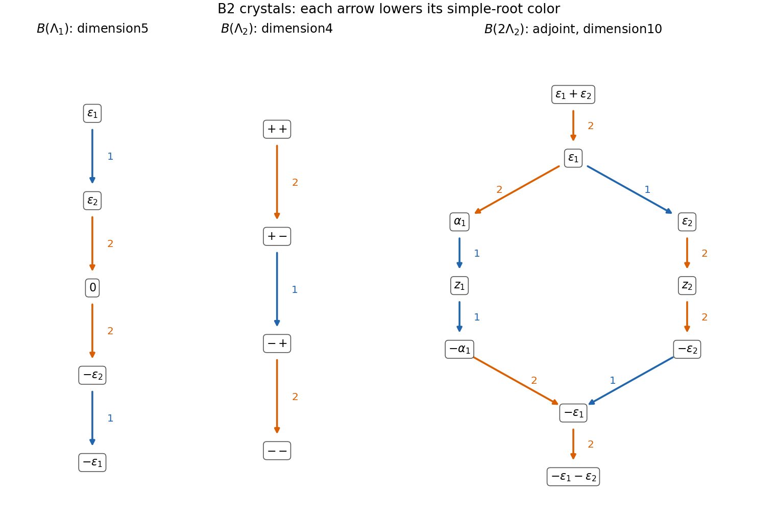
Codex 0 Created 2026-10-03 Updated 2026-10-14Use directed color- edges for the Kashiwara operator , so every edge subtracts from the weight. The defining crystal of the defining odd-orthogonal representation isThe defining module has highest weight and precisely these five weights, all of multiplicity one. The color-two string through zero has length two, since . The other indicated strings have length one. Restriction to each simple-root sl2 Lie algebra and the root-string property of a crystal justify the edges; no other weight difference is the relevant simple root.
For the B2 spin crystal , denote the four weights by their sign pairs. Its graph isThe fundamental weight is a minuscule weight: its pairings with all positive coroots are zero or one. Its Weyl orbit has four weights, and the dimension formula gives four, so each occurs once and there are no additional weights. All simple-root strings have length one. Subtracting or where another weight is present gives exactly this graph.
For the B2 adjoint crystal, write for the vertex of root weight , and use two distinct zero-weight vertices . There are eight root vertices and two zero vertices because the zero-weight space is the two-dimensional Cartan subalgebra. The complete lists of colored strings areEvery arrow in a given row has that row's color; the reverse arrows are the raising operators, and all unlisted lowering operations vanish. In particular the two zero vertices must not be merged.
For a constructive justification, let with the invariant symmetric form from part(a). The mapis an equivariant isomorphism , identifying the highest weight as . Compute its crystal as the highest-weight component starting at in , with labels for the defining chain. The crystal tensor-product rule iswhere counts available raising steps and counts lowering steps in the color- string. It generates the following ten vertices:Applying the displayed rule to these labels gives precisely the listed strings, proving the entire diagram rather than only its weight multiplicities. Tensor labels here are crystal vertices in the combinatorial limit, not an assertion that a bare ordinary tensor such as lies in .
Past exam of the mathematics course of the University of Cambridge 2001 iii Paper 5 2 c Solution by Codex 0 Created 2026-10-03 Updated 2026-10-14
Codex 0 Created 2026-10-03 Updated 2026-10-14Every finite-dimensional irreducible Lie algebra representation has highest weight for unique integers . The Weyl vector isso . In the Weyl dimension formula, the factors for the four positive roots, ordered as , are respectivelyHenceIn particular the two fundamental representations have dimensions five and four. The highest root is , so the Adjoint representation has dimension ten. These also fix the dimensions of the crystals below. Our numbering places the long root first; interchanging a B2/C2 numbering without interchanging the associated fundamental-weight labels would give the wrong dimension formula.
Past exam of the mathematics course of the University of Cambridge 2001 iii Paper 5 2 b Solution by Codex 0 Created 2026-10-03 Updated 2026-10-14
Codex 0 Created 2026-10-03 Updated 2026-10-14Give the real root span an inner product with orthonormal. The B2 root system consists of four short roots on the coordinate axes and four long roots on the diagonals. Choose the long-first simple rootsThe positive roots are , and . The corresponding simple reflections areThey generate every signed permutation of the two coordinates. Thus the Weyl group has order eight and is the symmetry group of a square; every element sends to or , with independent signs.
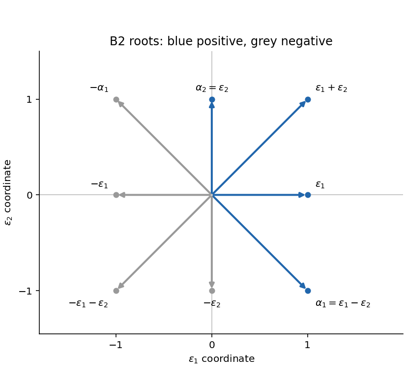
Since form an integral basis of , the root lattice is . The simple coroots are and . Therefore the weight lattice isSolving gives the fundamental weightsThe cone of dominant weights isIndeed and are exactly the two simple-coroot pairings. This describes representations of the Lie algebra, or of its simply connected Spin group; half-integral weights are allowed. For representations descending to itself, the weight must lie in , equivalently must be even.
Past exam of the mathematics course of the University of Cambridge 2001 iii Paper 5 2 a Solution by Codex 0 Created 2026-10-03 Updated 2026-10-14
Codex 0 Created 2026-10-03 Updated 2026-10-14The complex Special orthogonal Lie algebra consists of endomorphisms preserving a nondegenerate symmetric bilinear form infinitesimally:In an orthonormal basis this is , with the commutator bracket and dimension . Its compact real form is obtained by taking real skew-symmetric matrices. For diagonal root calculations it is more convenient to use an isotropic basis with , including .
A maximal torus of the complex special orthogonal group isIts Lie algebra is the Cartan subalgebraIn the compact real form the corresponding torus consists of independent rotations in two orthogonal coordinate planes, fixing the remaining direction. Define for , and , .
Writing for the matrix unit in the isotropic basis, lies in and satisfiesThus the nonzero root spaces are one-dimensional and the root-space decomposition isExplicit generators for four positive root spaces areThe transposes of these matrices generate the negative root spaces. Each transpose still satisfies the bilinear-form condition and reverses the displayed diagonal weight. These eight root vectors and the two independent Cartan matrices exhaust the dimension ten; a matrix commuting with every is diagonal and the form condition makes it lie in . This also proves that the torus has maximal dimension.
Past exam of the mathematics course of the University of Cambridge 2001 iii Paper 5 1 c Solution by Codex 0 Created 2026-10-03 Updated 2026-10-14
Codex 0 Created 2026-10-03 Updated 2026-10-14Apply the Weyl character formula with . In the Weyl denominator formula, replace every formal exponential by . This givesDividing by and cancelling each factor yieldsThe last expression is a compact way of writing the same character; individual half-root exponentials may need a larger formal lattice, but their full product lies in the group ring of the weight lattice. Expanding the first expression, a subset contributes the weight . Different subsets with the same sum give that weight's multiplicity. In particular , consistent with the Weyl dimension formula. This is the case of the character of a Weyl-vector multiple.
Past exam of the mathematics course of the University of Cambridge 2001 iii Paper 5 1 b Solution by Codex 0 Created 2026-10-03 Updated 2026-10-14
Codex 0 Created 2026-10-03 Updated 2026-10-14Let and identify the real weight and Cartan spaces using a Weyl group-invariant positive inner product. For a regular , meaning for every root, specialize to . Then the value of the formal character at is , but both Weyl alternants in the Weyl character formula vanish there. We compute their leading terms instead of substituting into that zero-over-zero expression.
ExpandFor every root reflection , replacing by changes the sign of , by replacing with in the sum. Replacing by also changes its sign, by replacing with . Thus the polynomial vanishes whenever or lies on any reflecting hyperplane. It is divisible by in its first variables and by in its second variables. Distinct positive roots give distinct linear factors; each product has degree .
The polynomial has degree in each group of variables. Therefore for , and for it has the formwith a constant independent of both variables. At , the Weyl denominator formula givesConsequently . For strictly dominant , its leading coefficient is nonzero, and the ratio of the two Weyl alternants tends toThe coroot is , so the root-length factors cancel in each ratio. This proves the Weyl dimension formula by the lowest-degree alternant proof of the Weyl dimension formula, including the limiting step.
Past exam of the mathematics course of the University of Cambridge 2001 iii Paper 5 1 a Solution by Codex 0 Created 2026-10-03 Updated 2026-10-14
Codex 0 Created 2026-10-03 Updated 2026-10-14Work over with a finite-dimensional semisimple Lie algebra . Choose a Cartan subalgebra , its root system , a positive system and its simple roots. Let be the Weyl group, generated by the corresponding root reflections, and put , the Weyl vector. The finite-dimensional irreducible highest-weight representation is indexed by a dominant integral weight .
If is the weight lattice, its group ring has formal symbols with multiplication . The formal character iswhere is a weight space. For a weight , define the Weyl alternant ; the sign is the determinant of on the real root span, equivalently the parity of its expression in simple reflections.
The Weyl character formula isThe second denominator is the Weyl denominator formula. The quotient can initially be taken in the fraction field of the group ring; the formula says it is the finite character on the left, so its apparent singularities are removable. The shifts by make strictly dominant.
Past exam of the mathematics course of the University of Cambridge 2001 iii Paper 49 3 c Solution by Codex 0 Created 2026-10-03 Updated 2026-10-14
Codex 0 Created 2026-10-03 Updated 2026-10-14For uniaxial extensional flow use , so . Again put and . A steady diagonal tensor hasSet . ThenSince and , multiplication givesThis is the cubic for uniaxial extension of an affine linear PTT fluid. For , choose its physical root , continuous from at rest. The product on the left grows strictly from zero to infinity in that interval, so this root is unique. The other algebraic roots need not describe an admissible steady material state.
The extensional viscosity is the axial-minus-transverse normal stress divided by the principal extension rate. Isotropic pressure cancels, leavingAt small , and . Thusthe Trouton ratio of three relative to the zero-shear viscosity. At large with fixed , the positive cubic root remains bounded and tends to : dividing the cubic by gives . ThereforeThe nonlinear relaxation prevents the divergent high-rate response of the affine Maxwell model. If , the physically stable steady branch instead has and ends at ; no finite positive high-rate limit follows. The finite plateau consequently presumes the usual positive PTT relaxation parameter, as well as .
Past exam of the mathematics course of the University of Cambridge 2001 iii Paper 49 3 b Solution by Codex 0 Created 2026-10-03 Updated 2026-10-14
Codex 0 Created 2026-10-03 Updated 2026-10-14Write and . With , the steady homogeneous upper-convected derivative is . Its diagonal and shear equations giveOn the physical branch , the other off-diagonal components vanish too. Thus , andFor the right side has derivative , so the shear stress determines a unique shear rate. The shear viscosity is and decreases with shear magnitude when . This is the shear part of shear and pipe flow of an affine linear PTT fluid.
For fully developed pipe flow take and the signed axial pressure gradient . Regularity at the axis and the supplied momentum balance determine the shear stress without using the constitutive equation:Locally the constitutive equations have the same shear form, with axial flow replacing the Cartesian flow direction and carrying its sign. HenceIntegrating and imposing no-slip boundary conditions at givesA negative pressure gradient produces positive axial flow. At this is the ordinary Hagen-Poiseuille flow; positive increases the flux at a fixed pressure drop through shear thinning. The nonzero axial normal stress varies radially, but its axial derivative vanishes in fully developed flow, so it does not change the axial momentum balance used here.
Past exam of the mathematics course of the University of Cambridge 2001 iii Paper 49 3 a Solution by Codex 0 Created 2026-10-03 Updated 2026-10-14
Codex 0 Created 2026-10-03 Updated 2026-10-14For the specified affine linear PTT fluid, perturb about the relaxed state , . Products of with the velocity gradient and the term are second order in the perturbation. The material-advection term is also second order. The linearized equation is thereforeWith vanishing stress in the remote past, an integrating factor givesSince , comparison with the linear viscoelastic fluid convolution yields and zero-shear viscosity . The nonlinear relaxation parameter does not appear at linear order; the response is that of a Maxwell fluid.
Past exam of the mathematics course of the University of Cambridge 2001 iii Paper 46 3 iv Solution by Codex 0 Created 2026-10-03 Updated 2026-10-14
Codex 0 Created 2026-10-03 Updated 2026-10-14On , the unperturbed trajectory satisfies . Put . Integration with givesIt runs from to , so it is the appropriate heteroclinic orbit. From the perturbed stream function,On the chosen connection, ; hence the scalar product in the heteroclinic Melnikov function for a periodic planar flow is . ThereforeSet . The odd term integrates to zero, leaving the supplied even Fourier integral multiplied by . ThusFor every fixed the amplitude is nonzero and the phase zeros are simple: there is . At fixed phase, varying also gives simple zeros because is nonzero for . The Melnikov splitting of a periodically perturbed cellular flow therefore produces transverse manifold intersections at sufficiently small perturbation and fluid-lobe exchange between adjacent cells. The unperturbed separatrix is no longer a material transport barrier.
At high frequency the leading splitting amplitude is asymptotic to , so fast forcing has an exponentially weak first-order effect on this connection. This is a fixed-frequency, small- result; an exponentially small leading term need not dominate higher orders in a simultaneous high-frequency limit. At exactly the perturbation itself vanishes and , so the nonzero-frequency conclusion does not apply. Manifold splitting demonstrates intercell chaotic advection locally, not a proof of uniform mixing or ordinary diffusion throughout the entire domain.
Past exam of the mathematics course of the University of Cambridge 2001 iii Paper 46 3 iii Solution by Codex 0 Created 2026-10-03 Updated 2026-10-14
Codex 0 Created 2026-10-03 Updated 2026-10-14Put and . Expansion of the trajectory equation to first order gives, for either correction,Since the unperturbed Hamiltonian flow obeys , differentiation with respect to position yields . Along the heteroclinic orbit this says . Therefore the homogeneous terms cancel:The unperturbed orbit approaches its hyperbolic fixed points exponentially, so at either appropriate endpoint. The selected stable and unstable corrections remain bounded there, approaching the first-order corrections to the periodic trajectories. Their endpoint dot products consequently vanish. Integrating the stable correction forward and the unstable correction backward givesSubtracting proves the heteroclinic Melnikov function for a periodic planar flow:Choose a regular point on the connection where . The first-order signed normal distance between the perturbed invariant curves is . If has a simple zero in the along-orbit parameter, the implicit function theorem continues it to a zero of the actual distance for sufficiently small , with nonzero derivative. The curves consequently cross transversely rather than touching tangentially.
A phase shift and a shift of the reference point along the autonomous connection are equivalent in this calculation: using changes the integrand from to . Thus a simple phase zero can also describe a crossing along the connection at a fixed forcing phase. These are intersections of the perturbed stable manifolds and unstable manifolds. The word “unperturbed” in the printed conclusion cannot be literal: those branches coincide before perturbation and have no transverse splitting.
Pinned article: Introduction to the OurBigBook Project
Welcome to the OurBigBook Project! Our goal is to create the perfect publishing platform for STEM subjects, and get university-level students to write the best free STEM tutorials ever.
Everyone is welcome to create an account and play with the site: ourbigbook.com/go/register. We belive that students themselves can write amazing tutorials, but teachers are welcome too. You can write about anything you want, it doesn't have to be STEM or even educational. Silly test content is very welcome and you won't be penalized in any way. Just keep it legal!
Intro to OurBigBook
. Source. We have two killer features:
- topics: topics group articles by different users with the same title, e.g. here is the topic for the "Fundamental Theorem of Calculus" ourbigbook.com/go/topic/fundamental-theorem-of-calculusArticles of different users are sorted by upvote within each article page. This feature is a bit like:
- a Wikipedia where each user can have their own version of each article
- a Q&A website like Stack Overflow, where multiple people can give their views on a given topic, and the best ones are sorted by upvote. Except you don't need to wait for someone to ask first, and any topic goes, no matter how narrow or broad
This feature makes it possible for readers to find better explanations of any topic created by other writers. And it allows writers to create an explanation in a place that readers might actually find it.
Figure 1. Screenshot of the "Derivative" topic page. View it live at: ourbigbook.com/go/topic/derivativeVideo 2. OurBigBook Web topics demo. Source. - local editing: you can store all your personal knowledge base content locally in a plaintext markup format that can be edited locally and published either:This way you can be sure that even if OurBigBook.com were to go down one day (which we have no plans to do as it is quite cheap to host!), your content will still be perfectly readable as a static site.
- to OurBigBook.com to get awesome multi-user features like topics and likes
- as HTML files to a static website, which you can host yourself for free on many external providers like GitHub Pages, and remain in full control

Figure 2. You can publish local OurBigBook lightweight markup files to either OurBigBook.com or as a static website.
Figure 3. Visual Studio Code extension installation.
Figure 5. . You can also edit articles on the Web editor without installing anything locally. Video 3. Edit locally and publish demo. Source. This shows editing OurBigBook Markup and publishing it using the Visual Studio Code extension. 
- Infinitely deep tables of contents:




All our software is open source and hosted at: github.com/ourbigbook/ourbigbook
Further documentation can be found at: docs.ourbigbook.com
Feel free to reach our to us for any help or suggestions: docs.ourbigbook.com/#contact