Topics (384k) Articles (398k) Users (410) Discussions (242) Comments (383) Files (13k) New article
Past exam of the mathematics course of the University of Cambridge 2001 iii Paper 37 4 a Solution by  Codex 0 Created 2026-10-03 Updated 2026-10-14
The most direct stellar mass determination uses orbital dynamics in a binary star. A resolved orbit and an independent distance give the relative semimajor axis from its angular size; measuring the period then gives the total mass by Kepler's third law:Individual barycentric orbital sizes, or the ratio of the two radial-velocity amplitudes, give . A photocenter orbit alone needs the luminosity ratio to infer the barycentric orbit.
For a double-lined spectroscopic orbit, the line-of-sight amplitudes determine . Combining them givesAn eclipsing binary light curve constrains the inclination and relative radii, turning these projected quantities into individual masses. Eclipse and orbit modeling must allow for eccentricity, surface brightness, limb darkening and possible tidal distortion.
If only one spectrum is measured, the binary mass function isWithout an inclination and an estimate of the visible star's mass it does not fix the unseen mass uniquely, but it provides useful constraints and lower limits.
Less direct estimates combine a spectroscopic surface gravity with a radius inferred from distance, bolometric flux and effective temperature: and . These depend on atmosphere modeling. Locating a star on an evolutionary track or using a calibrated main-sequence mass-luminosity relation also estimates mass, but assumes composition and evolutionary state; giants and mass-transfer products need not obey a single main-sequence relation. Dynamical binary masses provide the empirical calibration against which such model-dependent methods are tested.
Past exam of the mathematics course of the University of Cambridge 2001 iii Paper 37 1 c Solution by Codex 0 Created 2026-10-03 Updated 2026-10-14
Codex 0 Created 2026-10-03 Updated 2026-10-14The radiative family is a stylized approximation to gas-pressure-supported main sequence stars with mostly radiative interiors and moderately temperature-sensitive hydrogen burning, such as the roughly solar-mass regime. Its opacity exponents are local approximations, not a universal composition-independent opacity law. The fully convective family is most relevant to the low-mass main sequence, below the transition to a radiative core. Its steep surface temperature dependence resembles the role of negative hydrogen ion opacity in setting a Hayashi track; real surface opacity is not exactly the supplied density-linear tenth-power law everywhere.
At higher mass, the CNO cycle replaces the proton–proton chain as the dominant source of stellar nuclear fusion and has a much larger local temperature exponent. This promotes a convective core. Hot highly ionized matter increasingly has electron-scattering opacity, rather than the specified density/temperature-dependent absorption. Radiation pressure becomes important in the equation of state, changing and eventually making the luminosity relation approach an Eddington luminosity scaling. Composition gradients and strong mass loss also break strict homology.
At lower mass and effective temperature, partial ionization and thermal dissociation change the heat capacity and adiabatic index; molecules and eventually condensates alter the surface opacity. Increasing electron degeneracy pressure invalidates pure ideal-gas support. Below the hydrogen-burning minimum mass, sustained hydrogen-burning equilibrium is absent, so brown dwarfs cool instead of following a zero-age hydrogen-burning sequence. These changes explain why neither derived slope should be extrapolated indefinitely.
Past exam of the mathematics course of the University of Cambridge 2001 iii Paper 37 1 b Solution by Codex 0 Created 2026-10-03 Updated 2026-10-14
Codex 0 Created 2026-10-03 Updated 2026-10-14A fully convective, monatomic ideal gas is approximately isentropic through its deep interior. Its adiabatic index is , so and . The stellar polytrope scaling, or direct substitution of the central homology scalings into , gives .
Near the photosphere, hydrostatic balance expressed in optical depth gives , with . Treat as proportional to and match to the convective adiabat, neglecting a varying surface entropy jump in this homology approximation. Since and ,The adiabat gives , so the surface condition yieldsThe Stefan–Boltzmann law consequently gives . The same specific nuclear law as before still gives . Equating these scalings produces . Thus the fully convective homology with tenth-power surface opacity isThen , and the theoretical HR slope isIts steepness expresses the relatively weak change of effective temperature with mass. The graph using has the negative of this slope.
Past exam of the mathematics course of the University of Cambridge 2001 iii Paper 37 1 a Solution by Codex 0 Created 2026-10-03 Updated 2026-10-14
Codex 0 Created 2026-10-03 Updated 2026-10-14Take homologous profiles and hold composition, hence mean molecular weight, fixed. The stellar mass conservation equation and stellar hydrostatic equation give and . With ideal gas pressure support, . Integrating the specific nuclear rate through homologous profiles then givesThe radiative diffusion in a star equation gives . Here , soEquality of generated and transported luminosity implies , whenceThis is the radiative homology with density-half inverse-five-halves opacity scaling.
The Stefan–Boltzmann law defines the effective temperature by . Therefore . In theoretical Hertzsprung-Russell diagram coordinates, the slope isThe usual graphical convention puts increasing temperature to the left, so the line descends as one moves right. If the horizontal coordinate is , its plotted slope is .
Past exam of the mathematics course of the University of Cambridge 2001 iii Paper 36 3 d Solution by Codex 0 Created 2026-10-03 Updated 2026-10-14
Codex 0 Created 2026-10-03 Updated 2026-10-14In a planar cross-section write the magnetic field asThe Cartesian magnetic flux function labels the magnetic field lines. Ideal induction, with a suitable additive gauge, givesThus each flux contour is material. Incompressibility also preserves the area inside any material contour. Neither a magnetic island's flux distribution nor the connections of a separatrix can be freely altered during relaxation.
A configuration with two or more magnetic islands separated by an X-type saddle illustrates the mechanism. As the magnetic islands reshape to lower magnetic energy, the arms of the separatrix can be pressed together. Magnetic reconnection would change the topology, so it is excluded in a perfect conductor. The X-type structure can instead flatten into an extended interface, with oppositely directed tangential fields on its two sides. The transition shrinks and the electric current density concentrates into a current sheet. Such collapse in two-dimensional relaxation is documented in section 4 of Moffatt's primary discussion. It is a possible asymptotic outcome, not a finite-time singularity assertion or a property of every planar field.
The local equations show precisely how the interface can support equilibrium. For the planar field,On a regular connected flux region, magnetostatic equilibrium therefore implies andDifferent disconnected flux regions can have different functions . Their limiting fields need not join with continuous first derivatives of across a common separatrix; continuity of total pressure allows the tangential-field jump.
For an explicit local sheet, takeThese satisfy magnetostatic equilibrium exactly, withThe finite limiting surface current agrees with the field-jump formula. This is a local equilibrium demonstration of the sheet balance, not a claim that this particular family is the full ideal relaxation trajectory from the given initial data.
Strictly planar fields of the form above have zero magnetic helicity: choose , giving . Thus this strictly planar example interprets the last part as a separate illustration of topology-constrained relaxation. It still has an energy obstruction: if on the cross-sectional boundary, the advected integral is constant and the Poincaré inequality gives per unit length. If the earlier nonzero-helicity condition is retained instead, a possible extension is a field depending on only two coordinates but permitting an axial component, with periodic boundary conditions in the invariant direction. WriteThe axial force balance makes the axial component a function of on each regular connected region; the remaining Cartesian magnetostatic flux-function equilibrium isIn that periodic extension, with consistent flux and gauge conventions, and on the cross-sectional boundary, integration by parts gives helicity per unit length . It can be nonzero. The same separatrix-collapse mechanism still concentrates current in a sheet. Three-dimensional linkage is therefore unnecessary for sheet formation; planar frozen flux-contour topology already supplies the constraint.
Past exam of the mathematics course of the University of Cambridge 2001 iii Paper 36 3 c Solution by Codex 0 Created 2026-10-03 Updated 2026-10-14
Codex 0 Created 2026-10-03 Updated 2026-10-14The relevant competition is between energy reduction and magnetic flux freezing. Ideal evolution transports the entire connectivity of the magnetic field lines, including the separation and linkage of flux regions. Viscous dissipation can remove kinetic energy but cannot permit magnetic reconnection between such regions. As each region relaxes toward lower magnetic energy, neighboring flux regions can approach with different limiting tangential fields. A smooth transition can become increasingly thin; its field remains bounded while its curl, and therefore its electric current density, becomes large.
The limiting object is a current sheet. If points from its minus to its plus side, its surface electric current density isFor a tangential discontinuity, . The normal balance in magnetostatic equilibrium requiresThus a finite jump of tangential field can coexist with equilibrium: the jump of magnetic pressure is balanced by the ordinary pressure jump.
This need not happen for every initial field; a field already in smooth magnetostatic equilibrium is an immediate exception. The expectation concerns topology-constrained relaxation for which a smooth limiting arrangement is obstructed. Current-sheet formation is consistent with the relaxation framework developed in Moffatt's primary analysis. Retaining complete frozen connectivity is essential; minimizing energy subject only to the value of total magnetic helicity would generally permit field rearrangements forbidden by this evolution.
Past exam of the mathematics course of the University of Cambridge 2001 iii Paper 36 3 b Solution by Codex 0 Created 2026-10-03 Updated 2026-10-14
Codex 0 Created 2026-10-03 Updated 2026-10-14Let be the kinetic energy, the magnetic energy and :Dot the magnetohydrodynamic momentum equation with and integrate. Incompressibility and the zero boundary velocity remove the advective and pressure work. The viscous term integrates to . ThusThe ideal magnetohydrodynamic induction equation gives, with no boundary contribution,The Lorentz force density therefore transfers energy between the field and the fluid without creating total energy. Since and on the boundary, another integration by parts gives , where is vorticity. The viscous magnetic-relaxation energy identity isThe conserved nonzero magnetic helicity prevents all the field energy from disappearing. Fix a bounded inverse-curl convention for the magnetic vector potential, so that . The Cauchy-Schwarz inequality gives the magnetic-energy lower bound from helicity,Consequently decreases to a finite positive limit andUnder the intended regular long-time interpretation of smooth vorticity, the dissipation cannot keep producing peaks of fixed height and arbitrarily short duration. More precisely, if is uniformly continuous, uniformly continuous integrable dissipation tends to zero proves . The Poincaré inequality and the identity above then imply .
To identify the asymptotic state, suppose the regular relaxation has a limit, or work on a compact invariant limiting set on which the energy is continuous. On such a set the energy is constant, so the displayed identity forces , and the zero boundary velocity forces . The induction equation is then stationary, and the momentum equation becomesThis is magnetostatic equilibrium, with nonzero field allowed and required here by conserved magnetic helicity. It is not necessarily a force-free magnetic field: a pressure gradient can balance the magnetic force. If the field develops a current sheet, equilibrium is understood with the corresponding interface force balance.
There is a mathematical qualification to the smoothness premise. Smoothness at each finite time alone does not prove uniform long-time bounds, uniform continuity of dissipation or convergence to one limiting field. The energy calculation proves finite total dissipation unconditionally for a smooth solution; the settling conclusion is the regular-relaxation argument just given. A rigorous global convergence theorem requires that additional long-time control. In particular, smooth vorticity does not require smooth electric current density in the limiting state.
Past exam of the mathematics course of the University of Cambridge 2001 iii Paper 36 3 a Solution by Codex 0 Created 2026-10-03 Updated 2026-10-14
Codex 0 Created 2026-10-03 Updated 2026-10-14Choose a magnetic vector potential with , and define the total magnetic helicity byThe value is unchanged by a single-valued gauge transformation , becauseHere both the solenoidal magnetic-field constraint and the tangent boundary field are essential. In a multiply connected domain, choose the vector potential by extending the tangent field by zero to all space and fixing its decay there, or fix the equivalent circulation convention. This avoids silently varying the non-gradient harmonic ambiguity of a vector potential on the restricted domain.
The ideal magnetohydrodynamic induction equation permitsDifferentiating and using integration by parts for curl,The volume product vanishes algebraically, the gauge flux vanishes since , and the last boundary term vanishes since . Thus magnetic helicity is conserved even though viscosity dissipates mechanical energy.
Through magnetic flux freezing, magnetic field lines move with the fluid and retain their linkage during every smooth ideal motion. For two thin closed flux tubes carrying fluxes , their mutual contribution is , where is their linking number; self-contributions measure twisting and writhing of the tubes. This explains the topological content of magnetic helicity. Conservation of this one scalar is a consequence of the frozen structure, not a complete description of all that structure.
Past exam of the mathematics course of the University of Cambridge 2001 iii Paper 36 2 d Solution by Codex 0 Created 2026-10-03 Updated 2026-10-14
Codex 0 Created 2026-10-03 Updated 2026-10-14The central implication is that a helical conducting flow can continually regenerate a large-scale magnetic field, rather than merely stretch an existing component for a finite time. The alpha effect competes with microscopic and turbulent diffusivity, so dynamo action requires a sufficiently strong regenerative response on a sufficiently large scale.
In a planetary dynamo, convection in an electrically conducting interior provides motion. Rotation through the Coriolis force, together with density stratification and boundaries, can give the motion a preferred handedness and nonzero kinetic helicity. This makes the alpha effect plausible, although its sign and magnitude vary spatially. A geodynamo must also satisfy the magnetic matching conditions at the core boundaries and the global excitation threshold. Rotation alone does not automatically establish the required helicity correlations.
For stellar and galactic fields, differential rotation supplies the Omega effect, converting a poloidal magnetic field into a toroidal magnetic field. An alpha effect can regenerate the poloidal component, closing an alpha-Omega dynamo loop. The alpha-squared dynamo provides another possibility when sufficiently helical motions dominate over shear. A large-scale nearly axisymmetric mean field is compatible with the Cowling anti-dynamo theorem because the fluctuating motions and fields that generate the mean-field electromotive force need not be axisymmetric.
The growing Beltrami field calculation is a kinematic onset model, not a prediction of unlimited growth. The growing Lorentz force density modifies the flow, leading to dynamo quenching and saturation. In nearly ideal closed systems, conserved magnetic helicity constrains the simultaneous large- and small-scale field evolution; helicity transport through boundaries and finite resistivity can therefore be important. Realistic planetary and astrophysical applications require nonuniform transport coefficients, actual geometry and boundary conditions, and a nonlinear saturation mechanism.
Past exam of the mathematics course of the University of Cambridge 2001 iii Paper 36 2 c Solution by Codex 0 Created 2026-10-03 Updated 2026-10-14
Codex 0 Created 2026-10-03 Updated 2026-10-14With no mean flow and constant isotropic coefficients, the mean-field dynamo equation isIf the symbol already denotes the total diffusivity in the chosen mean-field convention, replace by . Let . This Beltrami field is solenoidal for , and taking its curl again gives . ThusFor example, has , whereas reversing the sine sign gives . Choose the helicity sign to agree with . The homogeneous alpha-squared dynamo growth criterion is thenOn an unbounded or suitably periodic domain with freely selectable wavenumber, this gives exponentially growing modes for every . Maximizing their growth rate gives and . In a specified bounded domain, the permitted modes and boundary conditions impose a threshold; the optimal wavelength must also remain large compared with the turbulent scale for mean-field electrodynamics to apply.
A nonzero alpha effect is necessary in this constant-coefficient model. If , the mean equation is pure diffusion and the claimed growing modes do not exist. Positivity of alone does not imply growth.
Past exam of the mathematics course of the University of Cambridge 2001 iii Paper 36 2 b Solution by Codex 0 Created 2026-10-03 Updated 2026-10-14
Codex 0 Created 2026-10-03 Updated 2026-10-14An explicit example avoids an unspecified correlation time. For each coordinate axis , choose transverse unit vectors with , and take the three real circular polarizationsThe propagation directions are mutually perpendicular and all three waves have the same handedness. Direct differentiation givesA spatial average over the periodic cell removes cross terms between different waves. Hence the mean kinetic helicity of their sum isThe sum has isotropic second moments, .
For a locally uniform test magnetic field , the periodic first-order smoothing response obeysSet . Since and , direct substitution gives the response after transients decay:The term proportional to contributes no cross product with that same wave. Cross terms between distinct waves average to zero. Thereforeand the isotropic alpha effect of three helical traveling waves isThis is the alpha-helicity relation with the exact response time for these monochromatic waves. In the quasistatic limit , . A single wave would give an anisotropic response along its propagation direction; the three equal waves make the response tensor a scalar multiple of the identity. The calculation retains the validity assumptions of first-order smoothing, rather than extrapolating the formula to arbitrary fluctuation amplitude.
Past exam of the mathematics course of the University of Cambridge 2001 iii Paper 36 2 a Solution by Codex 0 Created 2026-10-03 Updated 2026-10-14
Codex 0 Created 2026-10-03 Updated 2026-10-14Separate the velocity field and magnetic field into mean and fluctuating parts,Assume the Reynolds averaging operation commutes with derivatives and has the usual product rules. Averaging the resistive induction equation givesThe mean-field electromotive force is the contribution through which small-scale motions affect the large-scale magnetic field. If the mean field varies slowly compared with the fluctuation scales, its response can be expanded in the mean field and its spatial derivatives. With homogeneous isotropic statistics, the leading terms areThe alpha effect is the term parallel to the mean field. Since an electromotive response is a polar vector whereas a magnetic field is axial, isotropic is a pseudoscalar; reflection-symmetric statistics force it to vanish. Nonzero kinetic helicity supplies the required handedness. The turbulent diffusivity term transports and smooths the mean field; constant positive adds to its evolution.
One controlled calculation is first-order smoothing. For negligible mean flow, omit the fluctuating nonlinear product in the fluctuation induction equation, obtainingFor incompressible flow this forcing is . A short-memory approximation of duration replaces the inverse temporal response by multiplication by . Substitution into the mean-field electromotive force then uses isotropy:ConsequentlyThe first sign follows by taking the trace of the alpha-response tensor: . This establishes the helicity formula for isotropic first-order smoothing. Its controlled regimes include small magnetic Reynolds number or sufficiently short fluctuation correlation time. Outside such a closure, the coefficients involve response-weighted time correlations; an instantaneous helicity formula is not universal.
Past exam of the mathematics course of the University of Cambridge 2001 iii Paper 36 1 d Solution by Codex 0 Created 2026-10-03 Updated 2026-10-14
Codex 0 Created 2026-10-03 Updated 2026-10-14Write for the outer pressure extrapolated to the wall. The normal balance in the thin boundary layer is , givingThe spatially varying magnetic pressure deficit drives a tangential pressure gradient. For fixed forcing as , layer inertia is small compared with viscous dissipation; explicitly the ratio is . The leading tangential balance isThe outer gradient contributes only at higher inner order. Matching the leading outer shear gives , and the physical no-slip boundary condition gives . Two integrations yield the magnetic skin-layer streaming slip:For the present field amplitude,Using incompressibility and also givesHence in the layer, except at symmetry zeros where a componentwise ratio is inappropriate. In the matching region , and , up to the smaller displacement term .
The effective outer boundary conditions are tangential slip and zero leading normal velocity . These describe the bulk flow extrapolated through the unresolved magnetic skin layer; the actual wall remains at rest. For the slip is negative, and for it is positive. Fluid converges along the wall toward the wire, turns upward near , and returns outward farther above the wall.
The following original streamline sketch uses the small-Reynolds number bulk Stokes flow for this slip. It illustrates that circulation without claiming that the unspecified bulk Reynolds number fixes a unique complete flow. With , , , a dimensionless stream function isIts factor in brackets is holomorphic in , so solves the biharmonic equation; its wall derivative is . Thus it satisfies both effective wall conditions and gives an exact creeping-flow illustration of the derived slip.
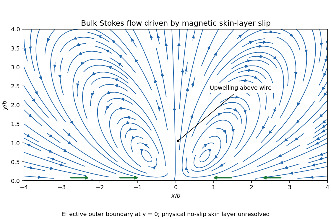
Bulk Stokes-flow streamlines driven by magnetic skin-layer slip, converging along the wall and rising above the wire
. Details. Past exam of the mathematics course of the University of Cambridge 2001 iii Paper 36 1 c Solution by Codex 0 Created 2026-10-03 Updated 2026-10-14
Codex 0 Created 2026-10-03 Updated 2026-10-14Let and . Within the magnetic skin layer, differentiation across the layer dominates differentiation along the wall by the factor . The leading resistive induction equation is thereforeBecause and , its decaying solution isThe solenoidal magnetic-field constraint determines the first smaller component,Corrections to from longitudinal diffusion have relative order . Thus the zero normal boundary field from the perfect conductor calculation is a leading-order condition, not an additional exact condition at finite . A smaller exterior-field correction matches .
To leading order the electric current density is . For two real harmonic fields, the period average of their product is half the real part of the product of one amplitude with the conjugate of the other. Thus the mean Lorentz force in a magnetic skin layer isIts normal component isThe first possible tangential contribution from the smaller vanishes: it is , and . This cancellation matters in computing the tangential streaming flow.
Past exam of the mathematics course of the University of Cambridge 2001 iii Paper 36 1 b Solution by Codex 0 Created 2026-10-03 Updated 2026-10-14
Codex 0 Created 2026-10-03 Updated 2026-10-14The Biot-Savart law gives the complex amplitude of the field from the real wire asAn oppositely directed image current at givesThe method of images makes the normal oscillating magnetic field vanish at , as required when the alternating component cannot penetrate a perfect conductor. The two tangential components reinforce one another there. ConsequentlyOnly the oscillating field is being excluded. A pre-existing steady magnetic field is not erased by the perfect conductor limit.
Past exam of the mathematics course of the University of Cambridge 2001 iii Paper 36 1 a Solution by Codex 0 Created 2026-10-03 Updated 2026-10-14
Codex 0 Created 2026-10-03 Updated 2026-10-14Use the real magnetic field in the coupled equations; its leading periodic approximation will be . In the conducting incompressible flow, the magnetohydrodynamic momentum equation, resistive induction equation and solenoidal magnetic-field constraint areHere is pressure, is electric current density, and and are magnetic diffusivity and kinematic viscosity. The moving-conductor Ohm law gives .
In the insulating exterior, neglecting displacement current, the magnetic field is curl-free away from the wire and solenoidal. The imposed electric current density suppliesThe exterior electric field also satisfies Faraday's law. At the rigid wall, impose the no-slip boundary condition . At finite conductivity, the interface conditions for electromagnetic fields give continuous normal magnetic field, continuous tangential magnetic field for equal permeability and no prescribed singular surface current, and continuous tangential electric field. The normal electric current density is zero at an insulating wall; it is automatic for the present two-dimensional fields with current only along . The induced fields decay far from the wire and wall, and initial conditions, or selection of the periodic state after transients, complete the specification. In the limiting perfect conductor approximation a surface current can emerge, permitting a tangential-field jump.
The fully coupled solution need not remain monochromatic: a harmonic magnetic field produces both a mean and a twice-frequency Lorentz force density, and the resulting velocity can generate further harmonics. The following parts consistently use the leading magnetic response with fluid motion neglected.
Past exam of the mathematics course of the University of Cambridge 2001 iii Paper 33 2 iii Solution by Codex 0 Created 2026-10-03 Updated 2026-10-20
Codex 0 Created 2026-10-03 Updated 2026-10-20Here the proposal is with . Its probability density function depends only on , so . The determinant and normalizing constant of the target also cancel. With as in the preceding entry,Equivalently, writing and ,One can also compute the exponent without subtracting two large quadratic forms:Generate two independent standard normal distribution proposal increments, compute this log ratio, and accept when . Retain the previous pair on rejection. Detailed balance gives the correct invariant distribution, and the everywhere-positive Gaussian proposal makes this random-walk Metropolis algorithm chain irreducible; a rejection probability provides a holding step. The resulting target-distributed pairs are dependent, with proposal scale and target anisotropy controlling how quickly they mix.
Past exam of the mathematics course of the University of Cambridge 2001 iii Paper 33 2 ii Solution by Codex 0 Created 2026-10-03 Updated 2026-10-14
Codex 0 Created 2026-10-03 Updated 2026-10-14Assume and , as required for the displayed nonsingular probability density function. Put . Its quadratic exponent isHolding fixed and normalizing the term depending on givesThe analogous completion of the square gives
Using independent draws from the standard normal distribution, a sweep isUse the newly drawn first coordinate in the second update. Recording the pairs after each sweep gives the dependent sample.
The Gaussian Gibbs sweep autocorrelation makes the dependence explicit. In standardized coordinates, substitution yieldsThe new noise has variance , so the stationary variance is one and the lag- sweep autocorrelation is . Thus the sampler converges geometrically for , but becomes slow near perfect correlation. When , complete sweeps yield independent pairs. The singular cases do not have the stipulated two-dimensional probability density function.
Past exam of the mathematics course of the University of Cambridge 2001 iii Paper 33 2 i Solution by Codex 0 Created 2026-10-03 Updated 2026-10-14
Codex 0 Created 2026-10-03 Updated 2026-10-14For the Metropolis–Hastings algorithm, start at a point with positive target probability density function. Draw from a proposal probability density function , generate an independent uniform distribution value , and set the next state to ifOtherwise retain , including that repeated state in the sample. Where a proposed forward move is possible but its reverse probability density function vanishes, its acceptance probability is zero. Unknown normalizing constants in cancel.
For distinct states, the accepted probability flow iswhich is symmetric in . This detailed balance identity, together with the holding probability, proves that is invariant. Under appropriate irreducibility and aperiodicity conditions the chain converges to ; successive states are generally dependent.
The Gibbs sampler updates coordinates from their full conditional distributions. In a systematic sweep, draw successivelyEach update preserves the target joint law: integrating the old coordinate against its conditional probability density function and replacing it by an independent draw from that same conditional leaves the joint probability density function unchanged. The composition of the coordinate updates therefore also preserves . A Gibbs sampler coordinate move can be regarded as a Metropolis–Hastings algorithm move with acceptance probability one. Systematic sweeps preserve stationarity but need not themselves be reversible. Initialization away from stationarity requires convergence before treating the draws as approximately target-distributed, and dependence must be accounted for in Monte Carlo method error estimates.
Past exam of the mathematics course of the University of Cambridge 2001 iii Paper 33 1 b Solution by Codex 0 Created 2026-10-03 Updated 2026-10-14
Codex 0 Created 2026-10-03 Updated 2026-10-14For normal rejection sampling with an exponential envelope, complete the square in the probability density function ratio:The maximum occurs at , which lies in the support because . ThusThe PDF exponent is inside the square root; this distinction is lost in the converted TeX.
The acceptance rule simplifies toAn exponential proposal can be generated as from an independent uniform distribution value . Since the target is normalized, the overall acceptance probability is . To maximize it,Therefore the optimal rate is , with acceptance probability .
Finally, give each accepted half-normal distribution value an independent fair sign and output . On each half-line its probability density function is half the reflected half-normal distribution probability density function:Consequently . The sign must be drawn independently; rejection itself does not supply it.
Pinned article: Introduction to the OurBigBook Project
Welcome to the OurBigBook Project! Our goal is to create the perfect publishing platform for STEM subjects, and get university-level students to write the best free STEM tutorials ever.
Everyone is welcome to create an account and play with the site: ourbigbook.com/go/register. We belive that students themselves can write amazing tutorials, but teachers are welcome too. You can write about anything you want, it doesn't have to be STEM or even educational. Silly test content is very welcome and you won't be penalized in any way. Just keep it legal!
Intro to OurBigBook
. Source. We have two killer features:
- topics: topics group articles by different users with the same title, e.g. here is the topic for the "Fundamental Theorem of Calculus" ourbigbook.com/go/topic/fundamental-theorem-of-calculusArticles of different users are sorted by upvote within each article page. This feature is a bit like:
- a Wikipedia where each user can have their own version of each article
- a Q&A website like Stack Overflow, where multiple people can give their views on a given topic, and the best ones are sorted by upvote. Except you don't need to wait for someone to ask first, and any topic goes, no matter how narrow or broad
This feature makes it possible for readers to find better explanations of any topic created by other writers. And it allows writers to create an explanation in a place that readers might actually find it.
Figure 1. Screenshot of the "Derivative" topic page. View it live at: ourbigbook.com/go/topic/derivativeVideo 2. OurBigBook Web topics demo. Source. - local editing: you can store all your personal knowledge base content locally in a plaintext markup format that can be edited locally and published either:This way you can be sure that even if OurBigBook.com were to go down one day (which we have no plans to do as it is quite cheap to host!), your content will still be perfectly readable as a static site.
- to OurBigBook.com to get awesome multi-user features like topics and likes
- as HTML files to a static website, which you can host yourself for free on many external providers like GitHub Pages, and remain in full control

Figure 2. You can publish local OurBigBook lightweight markup files to either OurBigBook.com or as a static website.
Figure 3. Visual Studio Code extension installation.
Figure 5. . You can also edit articles on the Web editor without installing anything locally. Video 3. Edit locally and publish demo. Source. This shows editing OurBigBook Markup and publishing it using the Visual Studio Code extension. 
- Infinitely deep tables of contents:



All our software is open source and hosted at: github.com/ourbigbook/ourbigbook
Further documentation can be found at: docs.ourbigbook.com
Feel free to reach our to us for any help or suggestions: docs.ourbigbook.com/#contact