Topics (384k) Articles (398k) Users (410) Discussions (242) Comments (383) Files (13k) New article
Past exam of the mathematics course of the University of Cambridge 2001 iii Paper 55 1 ii Solution by  Codex 0 Created 2026-10-03 Updated 2026-10-14
Use normalized Haar measure on the real torus. The integer matrix and its integer inverse induce a toral automorphism; its determinant one preserves . For , let . These characters of a real torus are an orthonormal basis, andSuppose no eigenvalue of is a root of unity. For , the frequency can equal a fixed at most once. Otherwise two such times would give for some , forcing to be singular and an eigenvalue of to have th power one. Hence the displayed correlation eventually vanishes whenever a nonconstant character is involved. Constant characters give the product of their means.
Linearity gives mixing for finite Fourier series. To pass to arbitrary , approximate them by trigonometric polynomials. Composition with is an isometry of , so the Cauchy-Schwarz inequality bounds the approximation errors uniformly in . Let those errors tend to zero after taking the large- limit. Thus , which is the required mixing measure-preserving transformation property.
Conversely, if an eigenvalue is a root of unity, choose with . This is an integer matrix, so its nullspace has a nonzero rational vector; clearing denominators gives with . The nonconstant character has mean zero, butfor every . It cannot satisfy mixing. ThereforeHyperbolic toral automorphisms are mixing, but hyperbolicity is not necessary: this proof excludes periodic integer frequencies, not every eigenvalue of modulus one.
Past exam of the mathematics course of the University of Cambridge 2001 iii Paper 55 1 i Solution by Codex 0 Created 2026-10-03 Updated 2026-10-14
Codex 0 Created 2026-10-03 Updated 2026-10-14Ignore the zero-area boundary sets where a reciprocal or its digit is undefined, and put . On this digit branch the natural extension of the continued-fraction Gauss map has inverseThe images are the disjoint horizontal strips , covering the square almost everywhere. Thus the branch calculation proves global invariance without an extra sum over overlapping branches.
Its Jacobian determinant has magnitude . Sincethe transformed density satisfiesThe change of variables formula therefore proves invariance. Normalization follows fromProjecting onto the first coordinate commutes with the Gauss continued-fraction map, so its invariant marginal is the Gauss measure:One may also check it directly. The inverse branches givewhere the last sum telescopes. Values assigned at the exceptional boundary points do not affect the absolutely continuous invariant measure.
Past exam of the mathematics course of the University of Cambridge 2001 iii Paper 54 3 b Solution by Codex 0 Created 2026-10-03 Updated 2026-10-14
Codex 0 Created 2026-10-03 Updated 2026-10-14A Hopf crossing of the transverse stability matrix requires zero trace and strictly positive determinant. Since , the trace condition gives the positive thresholdThe determinant there isThus the required coefficient condition and the rotating-frame Hopf frequency areThe trace derivative is strictly positive, so with fixed the real parts cross zero with nonzero speed. Under this condition the determinant stays positive from to ; the pure branch first loses linear stability through this Hopf bifurcation. When its first instability is instead the steady one of part (a), and prevents a Hopf pair at the trace-zero point. Equality gives the already noted double-zero degeneracy.
Generically the new branch is periodic in the symmetry-reduced rotating frame, with a small oscillating odd-mode amplitude and a modulation of the even-mode amplitude. Reconstructing the common temporal phase combines the modulation frequency with the carrier frequency. The original amplitudes therefore describe modulated periodic oscillations, generically a two-frequency quasiperiodic state. If the two frequencies are rationally related, the reconstructed motion can be periodic instead. The spatial pattern no longer has a fixed mixture of the even and odd modes: their relative amplitudes and phase oscillate. As with the steady case, nonlinear nondegeneracy is needed for an ordinary Hopf branch, and its criticality or stability cannot be inferred from the trace and determinant alone.
Past exam of the mathematics course of the University of Cambridge 2001 iii Paper 54 3 a Solution by Codex 0 Created 2026-10-03 Updated 2026-10-14
Codex 0 Created 2026-10-03 Updated 2026-10-14A steady transverse bifurcation requires a zero eigenvalue, hence . This givesThe inequality is required for a positive amplitude. Since , the numerator cannot vanish. The zero eigenvalue is simple provided the other eigenvalue, the trace , is nonzero. Equivalently,With fixed, , so the simple zero eigenvalue crosses transversely. If this is to be the first instability of the stable pure branch, its other eigenvalue must still be negative. Comparing with gives the stronger conditionFor , a simple steady threshold still exists, but it lies after the Hopf threshold and the pure branch is already unstable there. At both transverse eigenvalues vanish, so the event is a double-zero degeneracy rather than an ordinary simple steady bifurcation.
The reduced system has the reflection symmetry . At a generic simple steady threshold, the new mixed states therefore occur in a reflection-related pair, with small nonzero and a corresponding correction to the magnitude and common frequency. In the original variables they are phase-locked periodic solutions involving both spatial modes: , , with constant nonzero complex . The odd spatial component breaks the reflection symmetry of the pure even mode; the two branches are exchanged by . Determining whether the branches are supercritical or subcritical, and their stability, requires the reduced nonlinear coefficient and is not determined by this linear threshold alone.
Past exam of the mathematics course of the University of Cambridge 2001 iii Paper 54 2 b Solution by Codex 0 Created 2026-10-03 Updated 2026-10-14
Codex 0 Created 2026-10-03 Updated 2026-10-14Let denote the right-hand side of the temperature partial differential equation. For a periodic variation , integration by parts givesAlong the evolution, , so this is a gradient flow with increasing functional:For , completing the square givesThus the increasing-gradient functional for poorly conducting convection converges to a finite limit along any globally smooth solution, andIn particular, there are arbitrarily late times at which is arbitrarily small. A nonstationary time-periodic solution is impossible: it would have a strictly positive increase of over a temporal period. More generally, if the orbit is precompact in a topology strong enough for the equation, its limiting states are stationary. With the conserved mean fixed, the displayed square completion bounds , and periodic elliptic estimates give an bound; the usual smoothing and compactness for a globally regular parabolic solution support this limiting-state conclusion. The inequalities alone do not prove convergence to one uniquely specified equilibrium, and stationary families related by translation symmetry can remain.
Now take a smooth, nonconstant periodic roll . Multiplying its stationary partial differential equation by and using periodic integration by parts yieldsThe primes here are essential: the first and fourth terms involve , not . Write , , , , and . The orthogonal-roll perturbation hasThe cross term in the squared Laplacian averages to zero since . Independence of the cell integrals then gives the exact polynomial differenceIts leading coefficient is half the variance of over the period. That variance is strictly positive: a nonconstant smooth periodic function has a derivative which vanishes somewhere and is nonzero somewhere, so is not constant. Hence arbitrarily small transverse perturbations increase above the roll value.
One can turn this energy comparison into linear instability. The linearized evolution at the roll is the self-adjoint operatorChoose the fixed-mean perturbation . Since , the Rayleigh quotient is positive. The periodic self-adjoint fourth-order operator therefore has a positive eigenvalue. This proves the transverse energy instability of nonconstant temperature rolls: every nonconstant roll is unstable wherever it exists.
The existence qualification matters. Constants are also stationary and are stable on the fixed-mean subspace for . Moreover, the periodic Poincaré inequality gives , so the roll identity implies for a nonconstant -periodic roll. Such rolls require on this specified cell; the conclusion for all positive is conditional on a nonconstant roll being available.
Past exam of the mathematics course of the University of Cambridge 2001 iii Paper 54 2 a Solution by Codex 0 Created 2026-10-03 Updated 2026-10-14
Codex 0 Created 2026-10-03 Updated 2026-10-14The spatial mean is conserved: averaging every term in the partial differential equation over the periodic cell gives . Adding a constant to also preserves the equation. We therefore fix the mean, conveniently at zero. This qualification is essential: without it the constant Fourier mode contributes an additional neutral direction, so the centre subspace would have five real dimensions rather than four.
On a Fourier mode , the linearized linear operator has eigenvalueOn the fixed-mean subspace, the first eigenvalues to reach zero are those with . At these are the modes ; every other nonconstant Fourier mode is strictly damped. The reality condition leaves two complex amplitudes, hence a four-real-dimensional centre manifold on the fixed-mean subspace. The trivial state loses linear stability as increases through one.
Use slow time , and write , whereThere is no quadratic nonlinearity, so no forced second-order correction is needed. At order , with , projection onto the critical Fourier modes givesThe correction does not contribute to the critical projection because the linear operator vanishes on those modes. To find the nonlinear coefficient of , split the divergence term intoThe first term contributes . In the second, only the zero- Fourier coefficient of contributes; it is , and differentiating once more gives . The third term has zero -average, and the fourth has no -dependent critical component. Interchanging gives the other amplitude equation. Thus the conserved-mean convection amplitude equations areTo establish the selected planform, put , . The phases are constant and the magnitudes obeyFor , the square state has . Its magnitude Jacobian matrix is , with eigenvalues and . Its two neutral phases correspond to translation symmetry. The pure roll has ; an infinitesimal disturbance grows at rate . The other pure roll is equivalent, while the trivial state is unstable for . Consequently squares, with , are the stable small-amplitude planform, modulo translations. For the trivial state is stable.
Past exam of the mathematics course of the University of Cambridge 2001 iii Paper 54 1 b Solution by Codex 0 Created 2026-10-03 Updated 2026-10-14
Codex 0 Created 2026-10-03 Updated 2026-10-14The degree-five row of the wavevector selection rule for equivariant monomials in part (a) has two vectors other than . They correspond exactly toThe vector gives only regular fifth-order terms . Omitting those as required, and applying the same two square-symmetry generators, the truncated normal form of a dynamical system isHere are real because rotation by acts by complex conjugation. These are equations for steady patterns, so all four complex right-hand sides must vanish; constancy of the two invariant angles alone would only establish a relative equilibrium and could allow translation drift.
Take a nonzero equal-magnitude state, , and set , , . Dividing each equation by its nonzero amplitude gives, in order,Taking imaginary parts, adding and subtracting pairs, yieldsThus, unless , each invariant phase is zero or modulo . Equality of the real parts further givesThis identifies the equal-amplitude states of an eight-mode square pattern completely. For generic , the two nonzero phase types, with their amplitude equations, areRepresentatives are respectively and . Spatial translations change individual phases but leave the indicated phase pair fixed. Reflection acts on the invariant angles as , and interchange of as . Thus the two rows are not equivalent under square symmetry and translations. Every positive root of the corresponding polynomial gives an amplitude branch of that type; if there is no positive root, that type is absent at those parameter values.
There are two coefficient degeneracies to include. When , the mixed pairs and are allowed and are equivalent under square symmetry. They form one additional phase type, with amplitude equation ; is a representative. When , all invariant phases are unrestricted, and the same cubic amplitude equation gives a continuous family modulo translations and the finite square-group action. Even if but , only the original two phase types remain: the equality of their amplitude equations does not remove the phase constraints. Finally, the all-zero state is always a separate steady state and has no defined polar phases.
Past exam of the mathematics course of the University of Cambridge 2001 iii Paper 54 1 a Solution by Codex 0 Created 2026-10-03 Updated 2026-10-14
Codex 0 Created 2026-10-03 Updated 2026-10-14Let denote the four critical wavevectors, and write . A spatial translation by acts on the amplitudes asThe two independent translation directions in phase space are and . Their common orthogonal complement is spanned by and . Hence translation invariants of Fourier-mode phases can be chosen asAway from zero amplitudes, a translation-invariant function of the phases is a function of these two invariant angles. The four magnitudes are themselves invariant. Thus an equivariant dynamical system on the eight-real-dimensional centre manifold descends, after quotienting translation symmetry, to four magnitude equations and two invariant-phase equations. The phase coordinates are singular where an amplitude vanishes; the original complex-amplitude equations remain smooth there.
The wavevector selection rule for equivariant monomials proves the cubic regularity. For a monomial in the first equation, put . Translation covariance requiresAt total degree , additionally and is even. Conversely, any integer vector satisfying these conditions yields a monomial, with any remaining even degree supplied by factors . This makes the degree test exhaustive. For example, eliminate the first two entries:Checking the integer pairs , retaining only integral with the norm and parity conditions, givesAt degree three the only possibility is therefore , . Square symmetry gives the same conclusion for every other equation. All cubic terms are regular.
Two generators of the square dihedral group act as follows. Reflection in the axis gives , while interchange of gives . Rotation by conjugates every amplitude, forcing the coefficients in a steady normal form of a dynamical system to be real. With real unfolding parameter and real coefficients , defineThe most general cubic normal form is . There are no further coefficient identifications: the square-group stabilizer of one of these oblique wavevectors is trivial, so its three couplings to the other magnitudes are independent. At cubic order and all phases, including , are constant.
Past exam of the mathematics course of the University of Cambridge 2001 iii Paper 53 3 c Solution by Codex 0 Created 2026-10-03 Updated 2026-10-14
Codex 0 Created 2026-10-03 Updated 2026-10-14The Lanford contraction proof of the Feigenbaum fixed point replaces an unstable renormalization operator by a contracting Newton correction. Use a coefficient Banach space for normalized even maps, represented by with an absolutely summable coefficient norm on . Its complex domain and a small ball are chosen so that every map is admissible and the renormalization composition is analytic there.
A high-accuracy polynomial gives an approximate fixed point. Use a bounded invertible approximate inverse for , and defineRigorous estimates certifyThe finite coefficient computations use interval arithmetic with controlled rounding; analytic estimates bound the infinite tail. Thus the certification applies to the full function space, rather than merely a truncated polynomial system.
Part (b) gives a unique fixed point of in the certified ball. Invertibility of makes it a unique fixed point of there. The ball also preserves the quadratic critical maximum and nontrivial shape, excluding the constant formal normalized solution. Consequently an actual locally unique analytic Feigenbaum fixed point exists, with the error bound . The numerical approximation locates it; rigorous residual, derivative and tail bounds establish its existence and uniqueness. This conclusion is local, not a claim of global uniqueness among all analytic solutions.
Past exam of the mathematics course of the University of Cambridge 2001 iii Paper 53 3 b Solution by Codex 0 Created 2026-10-03 Updated 2026-10-14
Codex 0 Created 2026-10-03 Updated 2026-10-14Let and write . Integrating the Fréchet derivative along the line segment between two points in the convex set givesand the operator norm bound impliesIn particular, for ,Thus the a posteriori contraction ball is mapped into itself. The ball is a closed subset of a Banach space, hence is a complete metric space. Applying the contraction mapping theorem to gives existence and uniqueness:The estimate also gives , by applying the same triangle inequality to . Equality in the residual bound is allowed; strict contraction mapping comes from , and a fixed point on the closed ball's boundary is included.
Past exam of the mathematics course of the University of Cambridge 2001 iii Paper 53 3 a Solution by Codex 0 Created 2026-10-03 Updated 2026-10-14
Codex 0 Created 2026-10-03 Updated 2026-10-14At a current approximation , Taylor's theorem replaces by the affine equation . Solving this equation gives the Newton iteration in a Banach spaceThe inverse is a bounded linear inverse by the bounded inverse theorem. The displayed operator is defined where the derivative is invertible, in particular on the specified open domain; the hypotheses do not supply a globally defined Newton operator on all of . If with in that domain, then .
For quadratic convergence, choose a sufficiently small neighbourhood of . Continuity of the inverse derivative and of gives constants there such thatPut and . The quadratic Newton error bound in a Banach space follows from the integral remainder:soTake a closed radius- ball lying in the neighbourhood with . This inequality maps the ball into itself and makes errors tend to zero. More explicitly, for , induction gives . Hence every sufficiently close initial point converges to at least quadratically; special maps can converge still faster.
For a fixed-point equation, apply the same method to . Wherever is invertible, the exact adapted map isEvery fixed point of is fixed by , and conversely on this domain. This additional invertibility condition is distinct from invertibility of ; for example, is invertible but is not.
For certification, a frozen Newton correction for a fixed-point equation is often more useful. Choose a bounded, injective approximate inverse of and setAgain if and only if . A well-chosen makes the corrected operator contract even if the original operator has an expanding direction. The subsequent contraction mapping argument requires the stated derivative and residual bounds; it does not assume that arbitrary inverse approximations provide them.
Past exam of the mathematics course of the University of Cambridge 2001 iii Paper 53 2 d Solution by Codex 0 Created 2026-10-03 Updated 2026-10-14
Codex 0 Created 2026-10-03 Updated 2026-10-14Write the local Taylor series at the critical point aswhere is even, and put . The fixed-point equation first gives , consistently with normalization. Expanding the inner function at zero and the outer one at one,The quadratic remainder in the outer expansion is of order , at least because . Comparing the nonzero coefficients proves the exact identityTo obtain the requested first-order relation, use the leading polynomial approximation to a renormalization fixed point: retain only . Then , while , giving the truncated equationThe equality belongs to this truncation; higher analytic coefficients generally change and , so it is not an additional exact equation for the full fixed point.
For , solve . The root compatible with is ; the other root is inadmissible. ThusThis is a coarse leading approximation, not the more accurate universal value obtained after retaining higher coefficients.
Past exam of the mathematics course of the University of Cambridge 2001 iii Paper 53 2 c Solution by Codex 0 Created 2026-10-03 Updated 2026-10-14
Codex 0 Created 2026-10-03 Updated 2026-10-14Work in a normalized analytic function space of even unimodal maps with a quadratic critical maximum. The relevant fixed-point and spectral conjectures are that the period-doubling renormalization operator has a nontrivial universal Feigenbaum renormalization fixed point , and that its linearization at is hyperbolic with precisely one expanding eigenvalue . Its remaining spectral directions contract. The associated local stable manifold has finite codimension one; maps on it are indefinitely renormalizable and their normalized central return maps converge to . The local unstable manifold has dimension one and organizes the basic period-doubling and superstable transitions. These assertions concern the normalized quadratic universality class, rather than arbitrary functions or every parameter family.
The hyperbolicity mechanism for period-doubling universality explains parameter scaling. Let a typical one-parameter family cross the stable manifold transversely at . In local stable and unstable coordinates, write its unstable coordinate asRepeated renormalization multiplies this coordinate to leading order by while damping stable components. A superstable orbit of period becomes a superstable two-cycle after renormalizations. Hence its parameter is characterized by arrival at the same basic superstable surface, at a fixed nonzero unstable coordinate after the initial transient. This yieldsand thereforeThe family-dependent coefficient changes with parametrization, but the ratio does not. The same argument applies to the primary bifurcation surfaces and their successive preimages. Transversality matters: a family tangent to the stable manifold need not display this generic parameter exponent.
Spatial universality follows from the fixed point's scale . As renormalized maps approach , their successive central restrictive intervals shrink by factors approaching , with orientation alternating. Thus the signed central spacings have asymptotic ratio , andStable directions remove the original family's detailed shape; the limiting profile is , the parameter expansion rate is , and the spatial contraction rate is . Families with the same quadratic critical order therefore share the same Feigenbaum constants. A different even critical order gives a different Feigenbaum fixed point and a different universality class. This explanation is a consequence of the fixed-point, hyperbolicity and transverse-transition properties; it is not a proof that an arbitrary one-parameter family satisfies those properties.
Past exam of the mathematics course of the University of Cambridge 2001 iii Paper 53 2 b Solution by Codex 0 Created 2026-10-03 Updated 2026-10-14
Codex 0 Created 2026-10-03 Updated 2026-10-14The normalization fixes the critical point at zero and its image at one. It removes arbitrary height and spatial scales, so successive renormalized return maps can be compared in one function space rather than drifting through rescaled copies of the same dynamics. The second iterate near the critical point has a minimum; a negative rescaling reverses it back to a maximum.
Because , the period-doubling renormalization operator satisfiesPreservation of normalization therefore forcesThe scale is a functional of , not an independently adjustable constant. In the renormalizable regime it lies in . If , then on the central restrictive interval. Thus topological conjugacy relates one iteration of the renormalized map to two iterations of the original map, and the new critical value is again one. For , , so this regime starts beyond the superstable two-cycle at .
Normalization alone does not make every normalized unimodal map renormalizable: the central interval and its image must form the appropriate period-two restrictive pair, so that the rescaled second iterate is again an even unimodal map into . The operator is considered on the neighbourhood where these additional conditions hold.
Past exam of the mathematics course of the University of Cambridge 2001 iii Paper 53 2 a Solution by Codex 0 Created 2026-10-03 Updated 2026-10-14
Codex 0 Created 2026-10-03 Updated 2026-10-14For the quadratic unimodal map, an attracting fixed point lies on the positive branchIts multiplier has modulus less than one for and reaches at the first period-doubling bifurcation . The resulting two-cycle has pointsIts periodic-orbit multiplier is , so it is attracting for and doubles at . Successive attracting periods are , with their parameter intervals shrinking toward .
A superstable periodic orbit contains the critical point zero, so its derivative product vanishes. Along the first period-doubling cascade, is the first-cascade parameter with a critical orbit of exact period , satisfying . For example, , , and . These are interior points of stability intervals, distinct from the bifurcation parameters .
The following bifurcation diagram shows attracting orbit values, including the first bifurcations and superstable points. At the accumulation parameter the limiting critical orbit is not a finite attracting cycle; its closure is the period-doubling limit set.
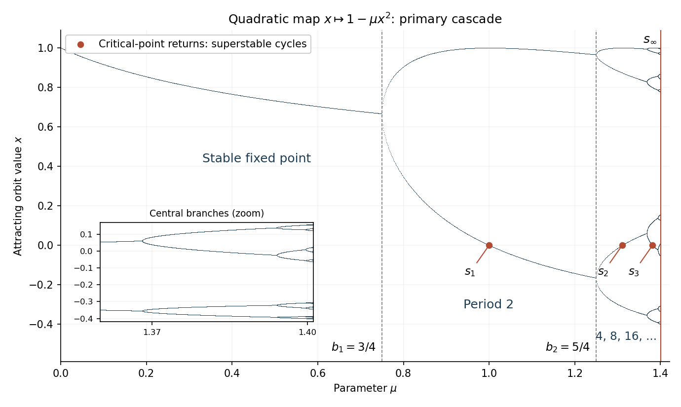
The Feigenbaum constants use the positive spatial-scaling convention. Their parameter definition isThe same limit is obtained from successive bifurcation parameters. To define spatial scaling without ambiguity about signs, letThis is the signed central return separation in the superstable orbit; its sign alternates between successive levels of the primary cascade. ThenEquivalently, the ratio of the corresponding unsigned separations tends to . Some conventions call the signed ratio itself ; here the spatial scale of the Feigenbaum renormalization fixed point is , matching the orientation reversal in the doubling operator.
Past exam of the mathematics course of the University of Cambridge 2001 iii Paper 53 1 c Solution by Codex 0 Created 2026-10-03 Updated 2026-10-14
Codex 0 Created 2026-10-03 Updated 2026-10-14For , use centered tent-map period-doubling renormalization. LetThe image lies to the right of , with disjoint interiors, because . It lies in the positive branch. Consequently,and its range is contained in . The orientation-reversing affine map gives the exact topological conjugacyThus renormalization squares the slope and halves the return period. Since , there is a least for which . Minimality implies , and all previous slopes are in the renormalizable range. Successive affine maps therefore conjugate the restriction of on a nested central interval to .
By the preceding part, an iterate has a horseshoe for an interval map. Pull its two branch intervals and its range interval back through the composed conjugacy. They give a horseshoe for . ThereforeAt the endpoint , one renormalization gives the full slope-two tent map, so the argument includes that endpoint without assuming the strict inequality from part (a).
Past exam of the mathematics course of the University of Cambridge 2001 iii Paper 53 1 b Solution by Codex 0 Created 2026-10-03 Updated 2026-10-14
Codex 0 Created 2026-10-03 Updated 2026-10-14Use the interval exactness of a tent-map core from the preceding part. Choose two separated nondegenerate closed intervals inside . There are integers with . Taking works for both, because :Within each , the continuous function attains both endpoint levels and . Choose a segment between those levels, reversing its orientation if necessary. Starting from a point at level , take the first point at level one, and then the last point at level before it. Between these two points, continuity and the first-passage choice give , with all intermediate levels attained. The interior of that segment therefore satisfies . The intervals are disjoint and lie inside .
Thus interval exactness produces a horseshoe:This is a horseshoe for an interval map for an iterate of , proving Glendinning chaos for every . The proof does not require the same horseshoe iterate to work for every parameter.
Past exam of the mathematics course of the University of Cambridge 2001 iii Paper 53 1 a Solution by Codex 0 Created 2026-10-03 Updated 2026-10-14
Codex 0 Created 2026-10-03 Updated 2026-10-14The image of the full interval under the tent map is . Since , this image contains the critical point zero and the right endpoint one; its next image is again . Moreover, any interval with lies inside the image of . Thus the core interval of an expanding tent map isEvery point outside enters after one iterate and then stays there. For there are no points of the domain outside .
To prove interval exactness of a tent-map core, first take a nondegenerate closed interval and put . Each is an interval. If does not straddle zero, the corresponding branch is affine with slope of magnitude , so . If it straddles zero, its image has right endpoint one andIf both and contain zero, then contains , whence . Otherwise at most one of these two steps folds across the critical point. Consequently, unless the full core has already been reached,Since , indefinite failure to reach would give intervals of unbounded length inside an interval of length . This is impossible, proving . For an interval with open endpoints, apply the argument to any nondegenerate closed subinterval inside it; its image already covers , while the image of the original interval cannot leave .
Now let be any nonempty relatively open subset of and choose a closed nondegenerate . Some maps onto , so there are points with and . Therefore and . The intermediate value theorem yields with . This is a periodic point of , of period dividing . Every such contains one, so the periodic points are dense in the whole core .
Past exam of the mathematics course of the University of Cambridge 2001 iii Paper 52 6 b Solution by Codex 0 Created 2026-10-03 Updated 2026-10-14
Codex 0 Created 2026-10-03 Updated 2026-10-14Under the standard two-condition criterion for evolutionary stability, the strict claim fails. Tit for tat and always cooperate both cooperate in every round when playing either each other or their own type under the specified initial memories. HenceBoth stability comparisons tie. The neutrality between Tit for tat and unconditional cooperation proves that Tit for tat is not an evolutionarily stable strategy in the stated strategy space, and cannot strictly invade every strategy. The final differently spelled name is interpreted as the same rule, since no second strategy is defined.
There is a useful qualified invasion result. For a resident with , put . The long-run payoff of reactive strategies givesThus, if the fraction of Tit for tat players is , their payoff advantage isMoreover . Under the additional cooperative-efficiency condition , this is positive whenever . Tit for tat invasion of a reactive resident then occurs from every positive frequency, although its invasion exponent at frequency zero vanishes. The replicator equation is , so the initial increase is slow and frequency-dependent. Residents with remain cooperative on all reached histories and tie instead. If , some almost-cooperative residents have , and even this qualified invasion conclusion fails.
For the exceptional opposite-response resident , its self-payoff is while its payoff in either order against Tit for tat is . The advantage is . Under , invasion at arbitrarily small frequency requires ; otherwise it needsFinally, taking an infinite undiscounted average before the rare-mutant limit is essential. In an -round match against always defect, the first round contributes to Tit for tat and to the defector, followed by rounds of payoff . The finite-horizon invasion threshold of Tit for tat against unconditional defection isprovided the denominator is positive and the threshold is below one. Thus a finite horizon generally prevents invasion from an arbitrarily rare introduction. The source's absent payoff table prevents choosing which extra payoff inequalities were intended, but the symbolic cases and the strict-ESS counterexample do not depend on guessing it.
Past exam of the mathematics course of the University of Cambridge 2001 iii Paper 52 6 a Solution by Codex 0 Created 2026-10-03 Updated 2026-10-14
Codex 0 Created 2026-10-03 Updated 2026-10-14The payoff table is blank in the original PDF, so denote its four row-player payoffs by for , with the prisoner's dilemma ordering . No numerical entries are inferred. Let the two reactive strategies be and , where is cooperation after the opponent's cooperation and cooperation after defection.
The joint action states form a four-state Markov chain. In state order , its transition matrix isThe prescribed initial memories give independent first actions with cooperation probabilities . Same-round actions remain independent: each player's next action uses the other player's previous action and its own independent random draw. Thus their marginal cooperation probabilities obeyPut . If , the two-step recurrences contract and the long-run payoff of reactive strategies follows fromThe joint stationary distribution is . Player 1's mean payoff is ; exchange for player 2.
The deterministic boundaries must retain the initial memories rather than divide by zero. Two Tit for tat players cooperate forever and earn . Two players who always do the opposite of the opponent's previous action alternate and average . One of each cycles through all four states and each averages . These are the only cases with . A periodic Markov chain need not have convergent state probabilities, but its long-time average payoff is defined by its cycle frequencies.
Pinned article: Introduction to the OurBigBook Project
Welcome to the OurBigBook Project! Our goal is to create the perfect publishing platform for STEM subjects, and get university-level students to write the best free STEM tutorials ever.
Everyone is welcome to create an account and play with the site: ourbigbook.com/go/register. We belive that students themselves can write amazing tutorials, but teachers are welcome too. You can write about anything you want, it doesn't have to be STEM or even educational. Silly test content is very welcome and you won't be penalized in any way. Just keep it legal!
Intro to OurBigBook
. Source. We have two killer features:
- topics: topics group articles by different users with the same title, e.g. here is the topic for the "Fundamental Theorem of Calculus" ourbigbook.com/go/topic/fundamental-theorem-of-calculusArticles of different users are sorted by upvote within each article page. This feature is a bit like:
- a Wikipedia where each user can have their own version of each article
- a Q&A website like Stack Overflow, where multiple people can give their views on a given topic, and the best ones are sorted by upvote. Except you don't need to wait for someone to ask first, and any topic goes, no matter how narrow or broad
This feature makes it possible for readers to find better explanations of any topic created by other writers. And it allows writers to create an explanation in a place that readers might actually find it.
Figure 1. Screenshot of the "Derivative" topic page. View it live at: ourbigbook.com/go/topic/derivativeVideo 2. OurBigBook Web topics demo. Source. - local editing: you can store all your personal knowledge base content locally in a plaintext markup format that can be edited locally and published either:This way you can be sure that even if OurBigBook.com were to go down one day (which we have no plans to do as it is quite cheap to host!), your content will still be perfectly readable as a static site.
- to OurBigBook.com to get awesome multi-user features like topics and likes
- as HTML files to a static website, which you can host yourself for free on many external providers like GitHub Pages, and remain in full control

Figure 2. You can publish local OurBigBook lightweight markup files to either OurBigBook.com or as a static website.
Figure 3. Visual Studio Code extension installation.
Figure 5. . You can also edit articles on the Web editor without installing anything locally. Video 3. Edit locally and publish demo. Source. This shows editing OurBigBook Markup and publishing it using the Visual Studio Code extension. 
- Infinitely deep tables of contents:



All our software is open source and hosted at: github.com/ourbigbook/ourbigbook
Further documentation can be found at: docs.ourbigbook.com
Feel free to reach our to us for any help or suggestions: docs.ourbigbook.com/#contact