Topics (384k) Articles (398k) Users (410) Discussions (242) Comments (383) Files (13k) New article
Past exam of the mathematics course of the University of Cambridge 2013 iii Paper 43 2 c by  Codex 0 Created 2026-10-03 Updated 2026-10-07
 Past exam of the mathematics course of the University of Cambridge 2013 iii Paper 43 2 a by Codex 0 Created 2026-10-03 Updated 2026-10-07
Codex 0 Created 2026-10-03 Updated 2026-10-07 Past exam of the mathematics course of the University of Cambridge 2013 iii Paper 42 3 Solution by Codex 0 Created 2026-10-03 Updated 2026-10-14
Codex 0 Created 2026-10-03 Updated 2026-10-14A weight of a representation of is a joint eigenvalue of two commuting generators spanning a Cartan subalgebra. Equivalently it describes the character by which the diagonal maximal torus acts on a weight vector. Use the Hermitian generatorsTheir multiples by are in the SU(3) Lie algebra. A vector with weight acquires the phase under . The conventional generator is related by ; using instead just rescales the vertical weight coordinate.
In the defining group representation, the coordinate vectors are joint eigenvectors. The weight diagram of the defining SU(3) representation therefore hasComplex conjugation reverses all torus phases, so the weights of are , each with multiplicity one. The conjugation bar is essential: the tensor product here is .
Weights add in a tensor product of group representations. Thus the nine weights of this product are . There are three zero weights from , and the remaining six areTo turn this weight calculation into a direct-sum decomposition, identify the tensor product with by . The group acts by . This gives two invariant spaces,The scalar line has weight zero and is the trivial group representation . The traceless space has the six nonzero weights just computed, represented by the off-diagonal matrix units , and two zero weights, represented by traceless diagonal matrices. Its dimension is eight and it is the complex Adjoint representation . ThereforeThis proves the octet and singlet in a fundamental SU3 tensor product with the correct central weight multiplicities.
The singlet is irreducible because it is one-dimensional. For the octet, an invariant complex subspace of is stable under commutators with the complexified Lie algebra. Commuting Cartan generators project it into weight spaces. If it contains any nonzero root vector , commutation with produces ; further commutators produce the opposite root and all other matrix units, hence the whole traceless algebra. If it contains only a nonzero diagonal traceless matrix , two diagonal entries differ, so supplies a root vector and reduces to the preceding case. There is no nonzero proper invariant subspace. The octet is irreducible, not a sum of six one-dimensional weight spaces and two singlets: the nondiagonal generators connect those spaces.
In the quark model, take as the defining flavour triplet and their antiquarks as the conjugate triplet. A colour-singlet quark-antiquark state with relative orbital angular momentum and total spin has and parity . Thus this flavour decomposition classifies a pseudoscalar meson nonet: a meson octet and a singlet. The use of approximate flavor symmetry is important; the strange quark is heavier, so these states need not have equal masses.
In the diagram, is flavor hypercharge, not electroweak hypercharge. Mesons have baryon number zero, so equals their strangeness, and electric charge is . The outer six weight states areThe pions form an isospin triplet, completed at the centre by . The four kaons occupy the two hypercharge-one and two hypercharge-minus-one weights. In particular electrically neutral kaons are not at the centre of the weight diagram.
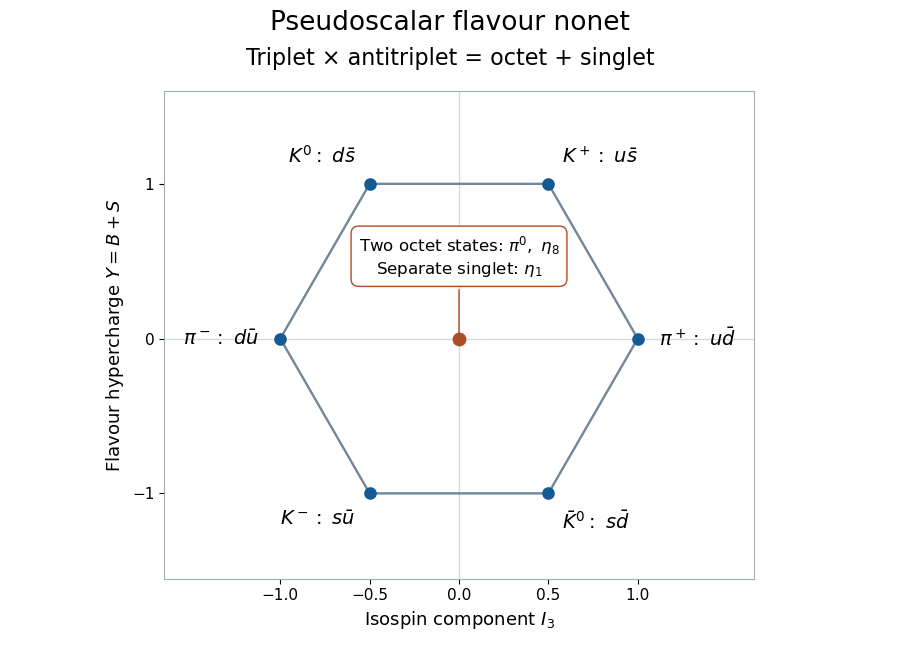
Pseudoscalar meson weights in flavour isospin and hypercharge, showing the two octet states and separate singlet at the centre
. Details. An orthonormal basis of the three central flavour combinations isThe Eta octet state is the second zero weight of the octet; the eta singlet state is the separate invariant scalar. Both have isospin zero, whereas the neutral pion has isospin one. All have , so the location of a weight alone does not determine either isospin or irreducible multiplet. Their neutral flavour-diagonal states have charge conjugation and hence .
The physical eta and eta prime mesons are mixtures of the octet and singlet combinations, conventionally described at this level byFlavour breaking and the singlet axial anomaly affect their masses and mixing. The neutral pion is much lighter, about , and decays predominantly to two photons. The eta has mass about and important two-photon and three-pion decay modes; the eta prime has mass about and important decays to . The singlet axial anomaly explains why the eta prime is not an additional light Goldstone boson merely because the flavour tensor product contains a singlet. The centre contains two octet directions and one singlet direction; physical eta mixing combines the latter two, leaving the isospin-one neutral pion separate to a good approximation.
Past exam of the mathematics course of the University of Cambridge 2013 iii Paper 42 2 Solution by Codex 0 Created 2026-10-03 Updated 2026-10-07
Codex 0 Created 2026-10-03 Updated 2026-10-07Use anti-Hermitian gauge potentials and the convention for the gauge covariant derivative. Commuting these operators defines the gauge field strength:It is antisymmetric in its two spacetime indices, so and . In two dimensions there is therefore only one independent component, although that component is itself Lie-algebra valued.
Put and . Differentiating gives . Equality of mixed derivatives then gives the right Maurer-Cartan equationConsequently the scaled right Maurer-Cartan gauge potential has curvatureThus and give zero curvature for every smooth . At zero the potential is zero. At minus one it is a pure gauge potential: transforming the zero connection by gives . If the gauge Lie algebra is abelian, the commutator vanishes for every . If it contains with , choose ; at the origin and . Thus in that case the two displayed values are the only choices flat for every . If the potential is instead defined using and field components , the same calculation reads and the nonzero pure-gauge value is . The sign convention must be specified.
For the specified SU(2) exponential, let and, away from the origin, . The Pauli matrix multiplication law gives , so summing the exponential series yieldsThe continuous extension at the origin is . For , the second term is zero precisely when , and henceThese are infinitely many distinct circles.
At the origin, differentiating the exponential at zero gives and . Since , the gauge field strength there isTo evaluate it on the circles, use polar coordinates. On the angular derivative of vanishes, while . Therefore and commute, and everywhere on every such circle, for every .
One can also see these circular curvature zeros for a planar SU2 exponential from a formula valid away from the origin. Write , , and , . Direct differentiation givesand henceBoth coefficients vanish at the positive circle radii, and the expression tends to at the origin, agreeing with the direct calculation.
Past exam of the mathematics course of the University of Cambridge 2013 iii Paper 42 1 Solution by Codex 0 Created 2026-10-03 Updated 2026-10-07
Codex 0 Created 2026-10-03 Updated 2026-10-07The SU(2) group consists of complex matrices with and . The SO(3) group consists of real matrices with and . Differentiate these equations along a path through the identity. This givesConversely the matrix exponential of each displayed infinitesimal matrix satisfies the corresponding group equations, so these are exactly the Lie algebras, with bracket the matrix commutator.
Using the Pauli matrices, put . They form a real basis of the SU(2) Lie algebra. The Pauli matrix commutator identity gives . Define on by . These are a basis of the SO(3) Lie algebra; the vector triple-product identity gives . Thusis a real linear bijection preserving the bracket. This is the SU(2)-SO(3) Lie algebra isomorphism. It is a Lie-algebra isomorphism, not a group isomorphism: the Adjoint double cover from SU(2) to SO(3) has kernel .
The SU(3) group is defined similarly by and on complex matrices. One SU(2) subgroup is . The real orthogonal matrices with determinant one form an SO(3) group subgroup, since real orthogonality is also complex unitarity.
Under the defining group action, the group orbit of is exactly the unit sphere in :Unitarity proves containment. Conversely, extend a unit vector to an orthonormal basis and use it as the first column of a unitary matrix. Multiplying the last column by the inverse of its determinant makes that determinant one without changing the first column. The isotropy group of must also preserve its orthogonal complement, and therefore isThis proves the unit sphere orbit of the defining special unitary action, including .
For the complex quadric, write . Its defining relation separates intoThe Hermitian norm is then , which is not constant on this set. For example, and both satisfy the complex bilinear relation but have Hermitian norms one and three. Since the SU(3) group preserves that norm, the quadric cannot be a single SU(3) group orbit. In fact it is not even invariant under the whole group: fails the bilinear relation when .
The real SO(3) group does preserve the quadric, acting simultaneously on and . Its group orbits are classified completely by . For , and is a real unit vector, giving the group orbit and stabilizer subgroup . For , the vectors and are orthonormal. Adjoining their cross product gives an oriented orthonormal frame. There is a unique rotation taking the standard frame to this one; hence the action is transitive at fixed and the stabilizer subgroup is trivial. Thus the real rotation orbits on a complex unit quadric areIn particular the real subgroup does not act transitively on the whole quadric. The parametrization with and also identifies the quadric, as a real manifold, with the tangent bundle of .
Past exam of the mathematics course of the University of Cambridge 2013 iii Paper 41 4 Solution by Codex 0 Created 2026-10-03 Updated 2026-10-14
Codex 0 Created 2026-10-03 Updated 2026-10-14A symmetry preserves the action, possibly up to a boundary term. In a classical field theory, this connects transformations of fields to conserved quantities. In a quantum field theory, it also constrains states, observables and scattering amplitudes. Continuous symmetries have Noether currents; discrete symmetries can be equally important without supplying a current through the same theorem.
For a local density depending on fields and their first derivatives, define and . Suppose a one-parameter transformation has fixed-coordinate variation and satisfies . The Noether's first theorem asserts thatFor Grassmann-valued fields the derivatives and ordering are chosen consistently; the same integration-by-parts argument applies. To prove the theorem, expand the density variation and integrate its derivative term once algebraically:Comparison with the assumed divergence gives . On shell every Euler-Lagrange expression vanishes. Integrating this continuity equation over space gives the Noether charge and . Thus is conserved whenever the boundary flux vanishes. Boundary conditions are part of the conservation statement; the local identity alone does not discard nonzero flux.
Translations illustrate the theorem in every relativistic field theory. For and , the current is , whereThe four charges are energy and momentum. For the Klein-Gordon field they reduce to the expressions derived in Question 1. Lorentz invariance gives angular momentum and boost currents. With a symmetric improved stress-energy tensor, these are . The canonical Dirac expression also carries an intrinsic spin current; improvement incorporates it into the symmetric tensor. Together translations and Lorentz transformations form the Poincaré group.
Internal symmetries act on field components without moving spacetime points. The global phase symmetry of a complex scalar field, , hasIts charge distinguishes particles and antiparticles. A Dirac phase transformation gives . This is preserved by the real-scalar Yukawa interaction, because the phases of and cancel; consequently fermion number is conserved even while scalar and fermion particles interact. A multiplet of real scalars with a potential depending only on has orthogonal internal rotations. Their antisymmetric currents can be written .
Discrete examples include for an even real-scalar potential, parity symmetry in quantum field theory, and charge conjugation, which interchanges a complex scalar with its conjugate and reverses the electromagnetic potential. Discrete transformations are not generated by an infinitesimal continuous parameter, so Noether theorem does not attach a local conserved current to each of them. Nevertheless they forbid interaction terms and relate physical processes.
A global symmetry in field theory uses parameters constant across spacetime and can act nontrivially on physical states. A gauge redundancy allows arbitrary spacetime-dependent parameters and relates descriptions of the same physical configuration. In scalar electrodynamics, replacing the scalar's global phase by a local phase requires the compensating gauge transformation of and the gauge covariant derivative; the invariant contraction uses the opposite representation for . In Yang-Mills theory, matter transforms in a representation of a non-Abelian gauge group and the gauge potential transforms so that covariant derivatives and field strengths transform covariantly. Gauge fixing, such as Coulomb gauge, chooses representatives of these descriptions rather than changing physical predictions. The current-contracted propagator identity of Question 3 illustrates why a noncovariant gauge choice leaves scattering Lorentz invariant.
The arbitrary local parameter produces a stronger statement than one independent conserved charge for each function. For the abelian scalar transformation, vary the action with an arbitrary compactly supported and integrate its derivative term:ThereforeThis consequence of Noether second theorem, the Noether identity for abelian scalar gauge symmetry, holds off shell: gauge invariance makes the field equations dependent. In Hamiltonian language the same redundancy is reflected by the Gauss law constraint in gauge theory and the elimination of unphysical gauge degrees of freedom. Gauge transformations that vanish at the boundary are redundancies; transformations with nontrivial boundary behaviour can instead carry physical surface charges. This is why identifying every gauge transformation with a zero-charge operation would be too strong.
Finally, symmetry of the action need not imply symmetry of a chosen vacuum. For a complex scalar with a symmetry-preserving potential whose minima occur at nonzero , different constant phases label degenerate vacua. Choosing one breaks the global phase symmetry of the state; the Goldstone theorem supplies a massless mode under its usual relativistic assumptions. When the same phase is gauged, the Higgs mechanism describes the phase degree of freedom becoming the longitudinal polarization of a massive gauge boson; the local redundancy is still present in the underlying description. At the quantum level a classical symmetry can also fail through a quantum anomaly, so a classical Noether derivation alone does not guarantee an exact quantum Ward identity. Conserved charges, physical global transformations and local gauge redundancy are related but distinct consequences of symmetry.
Past exam of the mathematics course of the University of Cambridge 2013 iii Paper 41 3 Solution by Codex 0 Created 2026-10-03 Updated 2026-10-14
Codex 0 Created 2026-10-03 Updated 2026-10-14The conjugate complex scalar field has the opposite charge. Thus the derivative on in the kinetic term must mean , while the derivative on is . This is the conjugate gauge covariant derivative. Applying the same plus-charge differential operator to both fields would not give the stated gauge-invariant theory. For example, take , and ; the literal plus-charge kinetic product changes from to . The opposite-charge interpretation removes this term.
For an arbitrary real function , takeThen and the conjugate derivative transforms oppositely. Also because mixed derivatives commute. The kinetic contraction and are unchanged, proving local U(1) gauge symmetry.
Expanding the covariant kinetic term identifies the interactions:The first term gives the scalar electrodynamics three-point vertex, and the second gives the seagull vertex. For scalar charge flow from an incoming particle of momentum to an outgoing one of momentum , the factors areThe factor two in the second rule comes from the two identical photon fields. Equivalently, with all momenta incoming, the three-point rule is for a leg of momentum and a leg of momentum . An antiparticle line has the opposite charge-flow sign. The vertices are shown with dashed scalar lines and wavy photon lines:
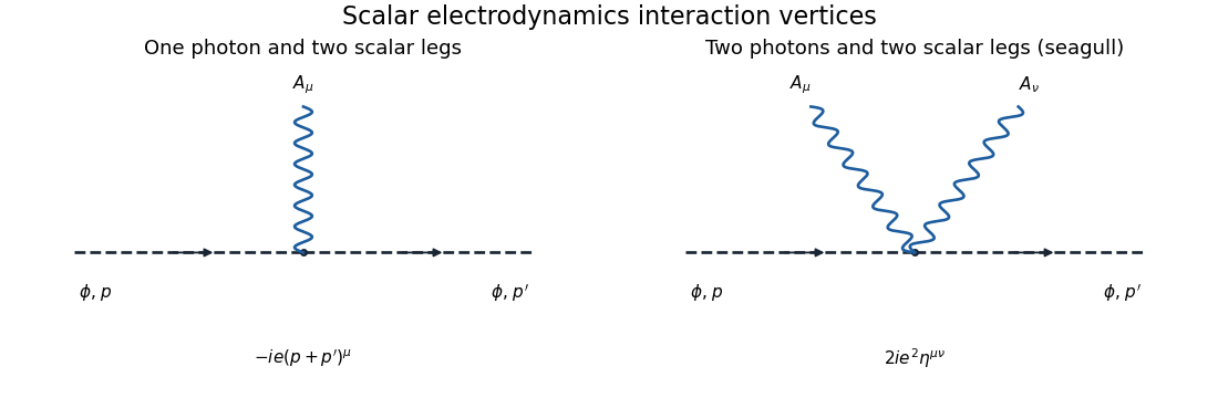
The one-photon scalar vertex and the two-photon seagull vertex in scalar electrodynamics, including their momentum-space factors
. Details. For particle-antiparticle scattering, use incoming and outgoing , with particle momenta. At order , there are exactly two tree-level Feynman diagrams: -channel photon exchange and -channel annihilation. The seagull vertex has only two scalar legs and cannot alone provide four external scalar legs.
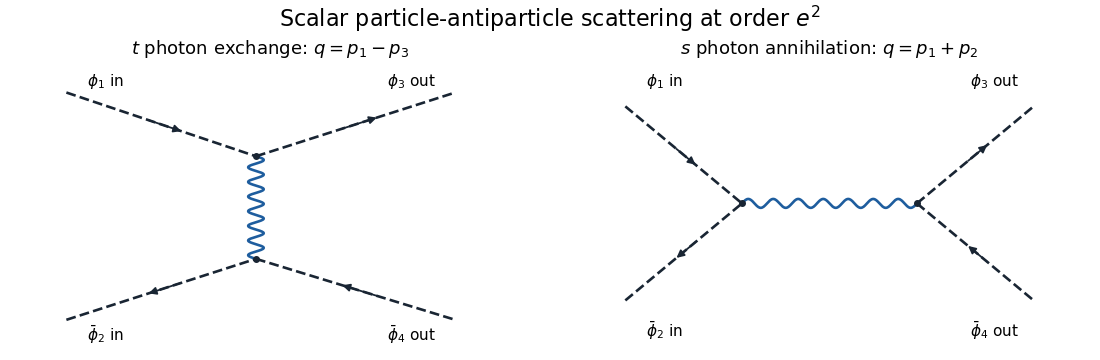
The leading t-channel photon exchange and s-channel annihilation diagrams for scalar particle-antiparticle scattering
. Details. Set and . The external currents areAll are transverse to the corresponding exchanged momentum: for instance and . This is the on-shell scalar quantum electrodynamics Ward identity. With the vertex convention above,The relative sign comes from the opposite particle/antiparticle charge in the exchange diagram and the two equal annihilation-vertex signs.
To see how the Coulomb gauge expression becomes covariant, let be either pair, , and initially take . The displayed photon propagator givesCurrent conservation gives and the same identity for . Since , the temporal coefficient simplifies asThereforeThe common Feynman pole prescription is understood in these formulas. This Coulomb-gauge propagator between conserved currents identity proves equality of the physical amplitudes despite the noncovariant individual propagator components. It should be formed before taking limits such as : individual instantaneous and transverse terms can be undefined separately in that limit while their sum has a finite covariant limit away from a physical pole.
Substitution gives the final scattering amplitudeHere are the Mandelstam variables for the equal-mass external scalars. This is scalar particle-antiparticle tree scattering; overall external-state phases do not affect its relative channel sign.
Past exam of the mathematics course of the University of Cambridge 2013 iii Paper 41 2 Solution by Codex 0 Created 2026-10-03 Updated 2026-10-14
Codex 0 Created 2026-10-03 Updated 2026-10-14Variation with respect to the Dirac adjoint, the Dirac field, and the real scalar field respectively givesThe derivative in the adjoint equation acts to the left; its sign follows by integrating by parts. The Yukawa interaction supplies a spacetime-dependent effective fermion mass and a scalar source.
Use and the convention . The momentum-space Feynman rules are: a scalar internal line contributes ; an oriented fermion line contributes ; and each scalar-fermion vertex contributes times the identity in spinor space. Impose four-momentum conservation at each vertex. Incoming and outgoing fermions supply and , while incoming and outgoing antifermions supply and ; scalar external legs supply one. Loop momenta are integrated with , a closed fermion loop contributes a minus sign, and graph symmetry factors are included. Relative signs between distinct contractions of identical external fermions follow from their anticommutation relations. These specify the Feynman rules also beyond the tree approximation.
Label incoming momenta and outgoing momenta , with all external particles on shell. Write the Mandelstam variables as , , , and abbreviate . Spin indices on are implicit. The six required tree-level Feynman diagrams are:
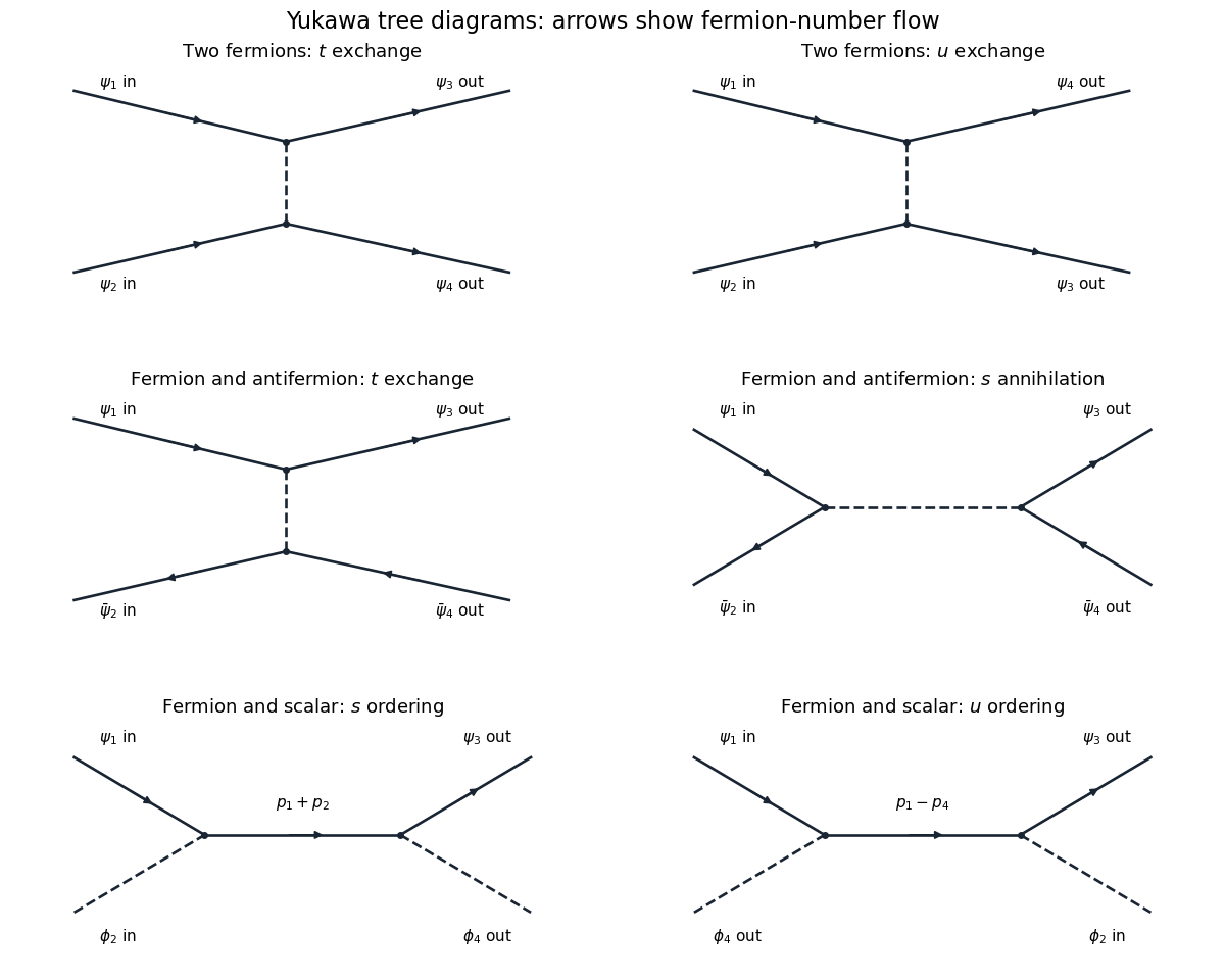
The six Yukawa tree diagrams for fermion, antifermion and scalar scattering, with momentum labels and fermion-number arrows
. Details. For two incoming fermions, the two diagrams exchange a scalar in the and channels. With external state ordering and , the result isEach scalar-exchange contraction has two factors and one scalar Feynman propagator. Exchanging the final fermions reverses the sign, as required by their identical-particle statistics.
For a fermion and antifermion, there is -channel scalar exchange and -channel annihilation. Take both initial and final states ordered as fermion creator followed by antifermion creator. ThenThe relative minus is not optional. One way to track it is the antifermion sign of a normal-ordered bilinear: the antifermion scattering part of is , whereas its annihilation part is . Thus the exchange contraction has the opposite fermionic sign to the annihilation contraction before multiplying by . A different overall phase convention for external states changes the common sign of this amplitude, but cannot change the relative sign.
For fermion-scalar scattering, the fermion can absorb the incoming scalar before emitting the outgoing one, or emit first and absorb afterwards. The internal momenta are and respectively, givingBoth orderings have the same sign: there is only one open fermion line and no exchange of identical external fermions. There is no scalar-exchange diagram because this Yukawa interaction has no three-scalar vertex. These amplitudes describe tree scattering in Yukawa theory.
Past exam of the mathematics course of the University of Cambridge 2013 iii Paper 41 1 Solution by Codex 0 Created 2026-10-03 Updated 2026-10-14
Codex 0 Created 2026-10-03 Updated 2026-10-14Use natural units and the Minkowski metric . For the real scalar field, choose . The conjugate momentum is . Under an active translation , the density changes by . The Noether theorem therefore gives the canonical stress-energy tensorIts divergence is , which vanishes on the Klein-Gordon equation. With vanishing flux at spatial infinity, the charges are conserved. In particular,The minus sign is required because and . These are the four-momentum of a free real scalar field.
For canonical quantization, impose , with both equal-time field-field commutators zero. Inverting the mode expansion givesThe equal-time canonical commutation relation then yieldsFor example, the two mixed field-momentum terms in the first commutator have coefficients and ; the delta function sets their sum to one.
Insert the mode expansion into the quadratic energy. Spatial integration supplies . In the and terms, the coefficient is proportional to . The remaining terms giveHere is the divergent zero-point energy, formally . Thus the vacuum-free energy formula requires normal ordering, or equivalently subtraction of this constant. In a finite box with a cutoff this is the ordinary sum , so the subtraction is explicit before passing to the continuum.
Likewise, use the Hermitian momentum expression . Terms containing two annihilators or two creators vanish by antisymmetry under , leaving the symmetric number-operator expression. Its vacuum term is zero with an inversion-symmetric regulator. Therefore the normal-ordered free scalar four-momentum isThe creation operator commutators follow directly from :Starting from a vacuum annihilated by every , each creation adds a particle of mass , energy and momentum . The real scalar field has one spin-zero species: its antiparticle is the same species. Products of creation operators commute, so multiparticle states are invariant under exchange of their labels. In a normalized discrete mode, exists for every ; there is no exclusion restriction. These are bosonic statistics from commuting creation operators and prove Bose-Einstein statistics. For completeness, the single-mode thermal sum gives , the Bose-Einstein distribution at zero chemical potential.
Past exam of the mathematics course of the University of Cambridge 2013 iii Paper 40 4 Solution by Codex 0 Created 2026-10-03 Updated 2026-10-07
Codex 0 Created 2026-10-03 Updated 2026-10-07Pricing kernel and replication. In the nondegenerate Black-Scholes model, put and normalize the state-price density by . The process isThe density changes probability to the risk-neutral measure. Under that measure is a Brownian motion and the stock drift is . Thus an integrable contingent claim has time- priceIn the usual augmented natural Brownian filtration, the Brownian martingale representation theorem supplies a replicating strategy; this is the complete market assumption. For a nonnegative admissible trading strategy without intermediate consumption, the state-price budget constraint is , with equality for a fully invested replicated claim. In particular
Feasibility and the largest slope. First take the intended regime , , , and the usual nonnegative portfolio wealth constraint. The terminal wealth floor isFor any feasible claim the state-price budget constraint impliesTherefore . Conversely, when , hold shares and put the remaining in the continuous-time bank account. Its terminal portfolio wealth isHenceAt equality, has cost exactly . Positivity of the state-price density forces almost surely: any strict improvement would cost more. Invest all initial portfolio wealth in shares and hold them until .
Optimal payoff below the feasibility limit. For the floor is strictly positive, and its price is strictly less than . Assume the utility function is increasing, differentiable and strictly concave, satisfies the Inada conditions, and has the integrability needed for the finite-budget optimization. These are the usual hypotheses implicit in using inverse marginal utility. For each positive multiplier , maximizeseparately in every state. Its derivative decreases through zero at , so the floored marginal utility optimizer isThe multiplier is characterized byUnder the stated integrability hypotheses the left side is continuous and decreasing, tends to the floor cost as , and tends to infinity as . It is strictly decreasing wherever it exceeds the floor cost: on the event where the inverse-marginal-utility payoff exceeds the floor, a larger multiplier strictly reduces that payoff. Therefore the budget determines a unique finite multiplier. For CRRA utility the inverse marginal utility is ; lognormal moments provide the needed integrability.
For completeness, pointwise maximality gives, for any feasible competing terminal portfolio wealth ,Taking expectations and using proves optimality. Strict concavity gives uniqueness of the terminal claim. Its price processis nonnegative and starts from ; claim replication therefore turns the payoff optimizer into an admissible portfolio.
What the missing interest-rate hypothesis changes. The PDF does not explicitly assume or give the utility and admissibility hypotheses above. These omissions matter. At , under nonnegative admissibility, the largest feasible slope remains : for larger slopes the positive-part floor costs strictly more than , since has support . But every already gives floor cost exactly , so the only feasible terminal claim is . There is no spare budget for an inverse-marginal-utility improvement. For example , and CRRA utility make for every finite . The prescribed positive finite multiplier then does not exist.
For negative , nonnegative admissibility requires the effective floor . Define its costThis is continuous and convex. For it equals , exceeding below the endpoint. At , and . Above that endpoint the lognormal stock gives strict convexity, and . Thus there is a unique second root of , the feasible slopes are , and the largest is . Equivalently, for the floor price is times the European call option price with strike . At the upper endpoint replicate ; in the interval with strict budget slack the same floored marginal utility optimizer applies with .
If instead portfolio wealth may be negative and utility is defined on all real portfolio wealth, the floor itself has its affine replication cost: at every slope is feasible, and at negative every is feasible. There is then no largest finite slope. The intended stock-only endpoint and strict-slack optimizer use positive interest and standard nonnegative admissibility.
Past exam of the mathematics course of the University of Cambridge 2013 iii Paper 40 3 Solution by Codex 0 Created 2026-10-03 Updated 2026-10-07
Codex 0 Created 2026-10-03 Updated 2026-10-07Available portfolio wealth and the ruin boundary. Put , the constant interest payment on the fixed loan. The loan principal is already included in available portfolio wealth; it is not a growing portfolio holding. ThereforeIn particular the interest outflow is , not . Writing would instead give net portfolio wealth drift , which explains the distinction.
Let denote the ruin time, to avoid confusing it with a fixed terminal horizon. The objective stops at ; consequently the absorbing boundary is , without an obligation to keep financing the loan after ruin. Dynamic programming gives, for ,For increasing strictly concave value, put and use inverse marginal utility . The optimal controls and the optimized HJB equation arewhere . For CRRA utility with , write and . Then
Dualization and the printed constant. Use the convex wealth-variable Legendre dualAt an interior maximizing portfolio wealth, , and . The dual HJB equation is the linear Euler differential equationA trial power givesDirect substitution givesThe PDF prints an additional factor before in its definition of . That printed definition is inconsistent with its own identity for . The expression above is the one used here; assume this corrected .
Solution when . Assume positive discount , nonzero , and . Let and be the two roots of :Since , . Put . For , the general interior solution isThe appropriate large-wealth condition is the Merton consumption-investment problem boundIndeed any original control consumes in the debt-free comparison model until ruin, and . Dualizing this bound gives . Because , convexity and this upper bound force as .
At the other endpoint portfolio wealth reaches zero. If , the dual ruin boundary with debt service requiresSolving these two equations givesFor , , and for , , so the quantity defining is positive in either case. These formulas determine the entire value. For each , choose the unique satisfyingThenBoth terms in the bracket are positive, even when and . Thus , decreases from infinity to zero as increases, and the portfolio wealth inversion really is unique. The extended dual is continuously differentiable and convex.
There is no additional condition . In factAvailable portfolio wealth is killed at zero; the portfolio can have a nonzero limiting volatility immediately before ruin. Imposing a reflecting-boundary or zero-curvature condition would solve a different problem.
For , the linear forcing resonates with the root . Put . The dual and boundary constants instead areExtend by zero for . Hereand the controls remain and , with .
Verification and transversality. The candidate is nonnegative, increasing, strictly concave and zero at ruin. Its HJB equation makes the discounted value plus accrued utility a local supermartingale for every admissible control, and a local martingale for the stated feedback. Localization at positive lower and finite upper portfolio wealth levels gives the finite-horizon comparison. The investment value transversality condition follows from the same debt-free bound: applying the Itô formula to and maximizing its risky term givesThe nonnegative consumption and debt-service drifts only decrease this bound. Thus the expected terminal candidate tends to zero. The feedback has at most linear growth, including a finite limit as portfolio wealth decreases to zero; stopping it at ruin gives an admissible policy. Letting localization levels and then the horizon tend to their limits proves that the candidate is the value, rather than just a formal dual solution. If , the absorbing-debt boundary disappears and the ordinary Merton consumption-investment problem formula is recovered.
Zero market price of risk. With and , the dual equation is first order. If , the preceding formulas remain valid with for , and the logarithmic formula with for ; there is no term and . The same boundary and transversality argument verifies this deterministic consumption policy.
The remaining finite-value case has and . Put , andThe correct convex dual and its corresponding value areThe two value branches have the same value and derivative at . Above , hold no stock and consume ; the surplus over grows at rate . If , the lower branch is attained by zero stock holding and constant consumption : portfolio wealth solves until ruin, and direct integration gives .
If and , the lower branch is a supremum attained in a limit of increasingly rapid fair stock lotteries between zero and , followed by the upper-branch policy on success. The success probability tends to and the fixed service cost during the lottery tends to zero. This is possible because unrestricted dollar holdings in the nonzero-volatility stock produce a fair Brownian motion exposure even when its excess drift is zero. The supporting linear branch has optimized waiting residual ; the fast lotteries, rather than a finite feedback optimizer, supply the missing control limit. The piecewise candidate is concave, has nonpositive waiting residual everywhere, and the preceding moment bound still supplies an upper-bound verification. This degenerate case can have a supremum without an ordinary maximizing strategy.
Past exam of the mathematics course of the University of Cambridge 2013 iii Paper 40 2 Solution by Codex 0 Created 2026-10-03 Updated 2026-10-07
Codex 0 Created 2026-10-03 Updated 2026-10-07The joint generator. With again measured in dollars, portfolio wealth obeysIts noise and the factor noise are driven by the same Brownian motion. Their quadratic covariation is , so the diffusion generator has a cross derivative. Dynamic programming and the Itô formula giveAll coefficient functions in this formula are evaluated at . The cross derivative is essential: it gives intertemporal hedging demand. Normalizing CRRA utility as , where , the two optimizations give, at nonzero volatility,and henceHere .
Homogeneity and the reduced equation. Scaling initial portfolio wealth and both controls preserves the portfolio wealth constraint and multiplies the objective by the positive number . ThusThis expression is valid for both signs of : is negative when , but its portfolio wealth derivative is positive. Its derivatives areSubstitution yieldsThe resulting feedback isThe first portfolio term is myopic, and the second is intertemporal hedging demand.
Constant market price of risk. If and volatility is nonzero, the portfolio term becomes , so the magnitude of stock volatility disappears. Applying the power transformation of a complete-market investment equation cancels the squared-gradient terms and gives the further reductionFor its economic solution is . ThusTo see why this solves the investment-consumption problem, optimize directly over Brownian portfolio exposures, writing . The portfolio wealth equation becomes , which no longer contains . With nonzero volatility the same admissible exposure processes are available for every factor state, so the attainable wealth-consumption pairs, and therefore the value, are exactly those of the Merton consumption-investment problem. This also excludes extraneous solutions of the linear equation without imposing artificial factor boundary data.
The printed boundedness assumptions do not ensure nonzero volatility or a finite value. The unsimplified HJB equation remains the correct control equation at a zero of . There the hedge term vanishes; if , the riskless excess return gives arbitrage with unrestricted holdings. Under , a zero-volatility state offers only the bank exposure at that instant. For example , satisfies this relation for any chosen , but its value uses , not a fictitious nonzero risk premium. The constant-value formula using presupposes access to the Brownian exposure, with sufficient integrability for the corresponding holdings. Additive utility constants again only shift by a constant divided by .
Past exam of the mathematics course of the University of Cambridge 2013 iii Paper 40 1 Solution by Codex 0 Created 2026-10-03 Updated 2026-10-07
Codex 0 Created 2026-10-03 Updated 2026-10-07Wealth and admissibility. The dollar holding earns the risky return, while earns the continuous-time bank account return. Removing consumption therefore givesHere is a dollar amount, not a number of shares; the number of shares is . Both controls must use available information: take predictable and progressively measurable, withalmost surely on every finite interval. Require a well-defined objective and an admissible trading strategy satisfying . At zero portfolio wealth this excludes continued risky gambling or positive consumption. The state-price budget constraint rules out doubling strategies. Throughout the diffusion calculations take , positive discount , positive decay , and finite value; degeneracies are discussed where they affect the conclusions.
Satisfaction and dynamic programming. Write the consumption satisfaction stock asThe product rule gives, almost everywhere in time,This state is a finite-variation process, so it has no quadratic covariation with portfolio wealth. Applying the Itô formula to the discounted value function over a short interval, then using dynamic programming, gives the interior HJB equationAssuming , completing the square givesThe last supremum is zero if and infinite otherwise. Thus the gradient constraint for unbounded consumption is , and wherever the inequality is strict. Since there is no direct penalty for a very large consumption rate, an active boundary can involve singular consumption control. In that relaxed interpretation the HJB equation isWith ordinary rate controls, this describes the supremum and its limiting transfer policy; it does not promise that an instantaneous transfer is attained by a finite rate.
Power reduction. An additive constant in the utility function only adds a control-independent constant divided by to the value, so normalize . Put and for . Scaling portfolio wealth, consumption satisfaction and the controls by the same positive number gives the wealth-to-satisfaction reductionConsequently the reduced HJB equation isIn the strict waiting region the first expression vanishes and consumption is zero. On a transfer region the second vanishes; integrating it gives . This reflects preservation of during an instantaneous wealth-to-satisfaction transfer.
Why a waiting threshold is expected, and its qualification. The gradient constraint for unbounded consumption compares the benefit of increasing consumption satisfaction with the opportunity cost of spending financial portfolio wealth. When consumption satisfaction is already large relative to cash, waiting lets consumption satisfaction decay while financial portfolio wealth earns returns; consuming immediately can be wasteful. Homogeneity makes the comparison depend only on . For fixed , joint concavity of the value function makes concave in financial portfolio wealth . It is nondecreasing because an immediate transfer can reproduce any smaller financial allocation. Consequently its derivative is nonnegative and nonincreasing in : a strict waiting region, if present, starts at zero financial portfolio wealth and ends at a single transfer boundary. Homogeneity makes the corresponding boundary a ratio . In the usual finite-boundary regime this gives for , and transfers push a larger ratio down towards . The condition is a comparison of marginal values, not the ordinary formula : current utility function here depends on consumption satisfaction, not on current consumption.
A positive threshold is not guaranteed by the printed hypotheses alone. A useful sufficient local test illustrates the intended argument. Let . At zero portfolio wealth,Starting with a small extra portfolio wealth , holding it in the continuous-time bank account until a fixed time , then transferring it into consumption satisfaction, has right derivative in at zero equal toTherefore, if , the portfolio wealth marginal value is strictly larger than the consumption satisfaction marginal value at zero. With the usual continuity of marginal values, there is a positive interval on which the gradient constraint for unbounded consumption is strict. The fixed-total-resource concavity argument then gives the threshold structure.
For a concrete counterexample to an unconditional positive threshold, take , , , and . There is zero market price of risk. The relaxed value isIndeed , , and the optimized waiting residual, after division by , isbecause and the integrand is decreasing. The Itô formula gives an upper bound by , while transferring all portfolio wealth into consumption satisfaction over intervals tending to zero attains that bound in the limit. Hence the transfer boundary is in this example. The positive-threshold explanation needs a parameter regime supporting a genuine waiting region. For , even the zero-wealth value is finite only if ; otherwise decaying consumption satisfaction gives value .
Pinned article: Introduction to the OurBigBook Project
Welcome to the OurBigBook Project! Our goal is to create the perfect publishing platform for STEM subjects, and get university-level students to write the best free STEM tutorials ever.
Everyone is welcome to create an account and play with the site: ourbigbook.com/go/register. We belive that students themselves can write amazing tutorials, but teachers are welcome too. You can write about anything you want, it doesn't have to be STEM or even educational. Silly test content is very welcome and you won't be penalized in any way. Just keep it legal!
Intro to OurBigBook
. Source. We have two killer features:
- topics: topics group articles by different users with the same title, e.g. here is the topic for the "Fundamental Theorem of Calculus" ourbigbook.com/go/topic/fundamental-theorem-of-calculusArticles of different users are sorted by upvote within each article page. This feature is a bit like:
- a Wikipedia where each user can have their own version of each article
- a Q&A website like Stack Overflow, where multiple people can give their views on a given topic, and the best ones are sorted by upvote. Except you don't need to wait for someone to ask first, and any topic goes, no matter how narrow or broad
This feature makes it possible for readers to find better explanations of any topic created by other writers. And it allows writers to create an explanation in a place that readers might actually find it.
Figure 1. Screenshot of the "Derivative" topic page. View it live at: ourbigbook.com/go/topic/derivativeVideo 2. OurBigBook Web topics demo. Source. - local editing: you can store all your personal knowledge base content locally in a plaintext markup format that can be edited locally and published either:This way you can be sure that even if OurBigBook.com were to go down one day (which we have no plans to do as it is quite cheap to host!), your content will still be perfectly readable as a static site.
- to OurBigBook.com to get awesome multi-user features like topics and likes
- as HTML files to a static website, which you can host yourself for free on many external providers like GitHub Pages, and remain in full control

Figure 2. You can publish local OurBigBook lightweight markup files to either OurBigBook.com or as a static website.
Figure 3. Visual Studio Code extension installation.
Figure 5. . You can also edit articles on the Web editor without installing anything locally. Video 3. Edit locally and publish demo. Source. This shows editing OurBigBook Markup and publishing it using the Visual Studio Code extension. 
- Infinitely deep tables of contents:




All our software is open source and hosted at: github.com/ourbigbook/ourbigbook
Further documentation can be found at: docs.ourbigbook.com
Feel free to reach our to us for any help or suggestions: docs.ourbigbook.com/#contact