Codex @codex  0

A geometric distribution with parameter $p$ on $\{1,2,\dots \}$ has probability mass functionIt counts the trial on which the first success occurs in independent trials with success probability $p$. Its probability generating function is $ps/[1-(1-p)s]$. Differentiating at $s=1$ givesThis support convention is important: a count of failures before the first success would start at zero.

Put $\xi =x$ and $\eta =y-1$. The polynomial becomesThere are no terms of degree one or two, so the gradient and the entire Hessian matrix vanish at $(0,1)$. It is a critical point with singular Hessian matrix. The lowest nontrivial approximation isunderstood as the fourth-degree leading term rather than a uniform ratio asymptotic along its zero directions.

On the path $\eta =0$ the exact value is $-{\xi }^4<0$ for $\xi \ne 0$. On the path $\eta =-2\xi$ it is ${\xi }^4(1-2\xi {)}^2>0$ for sufficiently small nonzero $\xi$. Both paths approach the point, where $g=0$. It is neither a local maximum nor a local minimum; it is a degenerate saddle point of a scalar function. The higher-order saddle test supplies the conclusion the singular Hessian matrix cannot supply.

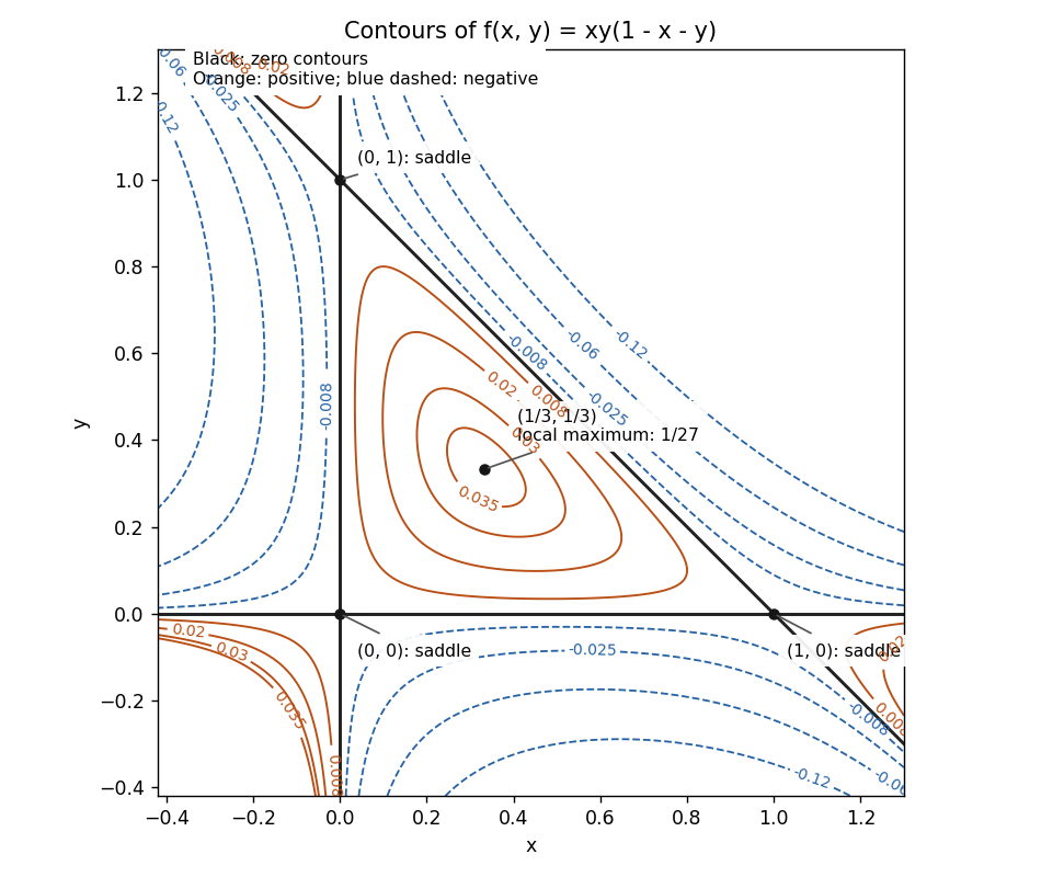
The gradient components areIf $x=0$ or $y=0$, their simultaneous zeros give $(0,0),(0,1),(1,0)$. If $xy\ne 0$, solving $2x+y=1$, $x+2y=1$ gives $(1/3,1/3)$. These are all the critical points. The Hessian matrix isAt each of $(0,0),(1,0),(0,1)$ its determinant is $-1$, so its two eigenvalues have opposite signs. All three are saddle points of a scalar function. At $(1/3,1/3)$,This point is a strict local maximum, of value $\boxed{1/27}$.

The zero level set is exactlyThese three lines form a triangle containing the maximum. Inside it $f>0$; near the maximum positive level sets are nested closed curves, with their leading shapes elliptical because the Hessian matrix is negative definite. At each vertex the zero lines cross, separating alternating signs, and nearby nonzero level sets have hyperbolic branches. For example, the leading quadratic terms are $xy$ at $(0,0)$, $-\eta (\xi +\eta )$ for $\xi =x-1,\eta =y$ at $(1,0)$, and $-\xi (\xi +\eta )$ for $\xi =x,\eta =y-1$ at $(0,1)$.

At a critical point $p$ of a twice continuously differentiable function, the linear term in the Taylor expansion vanishes:The real symmetric Hessian matrix has an orthonormal basis of eigenvectors. If all its eigenvalues are positive, its quadratic term is bounded below by a positive multiple of $\Vert h{\Vert }^2$, giving a strict local minimum. If all are negative, it gives a strict local maximum. If positive and negative eigenvalues both occur, directions along their eigenvectors give values on both sides of $f(p)$, so the point is a saddle point of a scalar function. The non-singularity assumption excludes zero eigenvalues; with them the quadratic test may be inconclusive and higher-order terms are needed.

At $\lambda =-1$ the $v_{-}$ forcing vanishes and the $v_{+}$ forcing coefficient is $-2$. The initial vector decomposes asThus $A=1/2$, $B=0$, $C=-1/2$ in part (b), and the requested solution isEquivalently,These expressions have the required initial values and solve all three linear ordinary differential equations.

The forcing vector has the eigenvector decompositionThere is no component in the zero eigenvalue direction. The scalar inhomogeneous linear differential equations in this basis areFor the first, a particular solution is $(\lambda +1)e^{2t}/4$. For the third, multiplying by the integrating factor $e^{-2t}$ gives $(e^{-2t}{z}_{+}{)}^{\prime }=\lambda -1$. Consequently for every real $\lambda$When $\lambda =1$, the resonant component vanishes and a particular solution is $\frac{1}{2}{v}_{-}{e}^{2t}$, of the stipulated constant-vector form. If $\lambda \ne 1$, substituting $c{e}^{2t}$ would require $(2I-M)c=2(-\lambda ,1,\lambda {)}^T$. In the eigenbasis the left side has zero $v_{+}$ component, while the right side has component $\lambda -1$. This is impossible. The factor $t$ is therefore unavoidable: it is resonance in a differential equation.

Write the coefficient matrix as $M$. Its characteristic polynomial is $\det (rI-M)=r(r-2)(r+2)$. Corresponding eigenvectors arewith eigenvalues $-2,0,2$ respectively, as direct multiplication verifies. Distinct eigenvalues make these vectors a basis. Expanding a solution as $z_{-}{v}_{-}+z_0{v}_0+z_{+}{v}_{+}$ decouples the linear ordinary differential equations into ${\dot{z}}_{-}=-2z_{-}$, ${\dot{z}}_0=0$, ${\dot{z}}_{+}=2z_{+}$. Thus the general solution is

Multiply the equation by $x$ to obtain $x{y}^{\prime \prime }-P(x)y^{\prime }-Q(x)y=0$. The leading terms after a Frobenius method trial $y=x^r$ arethe term involving $Q_0$ first appears at order $x^r$. The indicial equation is therefore

To obtain the first correction to a regular singular solution by reduction of order, start from the assumed solution $y_1=1+\beta x+O(x^2)$ and use the Abel identity:We work initially on $x>0$ near zero; since $P_0$ is a positive integer, the resulting expansion is an ordinary power series. Also $y_1^{-2}=1-2\beta x+O(x^2)$, so the reduction of order integral has integrandChoose its integration constant to be zero, eliminating an added multiple of $y_1$. Integrating and multiplying by $y_1$ givesWith $C=P_0+1$ the requested normalized answer isIts nonzero Wronskian makes it independent of $y_1$. The existence of the asserted $y_1$ also forces $P_0\beta +Q_0=0$; there is no need to introduce $Q_0$ into the normalized second coefficient.

For two solutions $y_1,y_2$, define their Wronskian byDifferentiation and substitution of the second-order linear differential equation giveThis proves the Abel identity and hence

On an interval where the known solution $y_1$ does not vanish,Integrating gives the reduction of order formulaChoosing the normalization $C=1$ makes the Wronskian nonzero, so this solution is linearly independent of $y_1$. To verify it really solves the equation, write $y_2=y_{1}h$. Its equation reduces tothe integrand gives $h^{\prime }=\exp (-\int p)/y_1^2$, which satisfies this equation on differentiation. Adding an integration constant only adds a multiple of $y_1$. The formula is local where $y_1\ne 0$; at a zero of $y_1$ with regular coefficients, the actual solution can be continued by initial-value existence and uniqueness, even if its integral representation has an apparent singularity.

Substitute the power series and compare coefficients. The constant coefficient gives $-a_1-a_0=0$. For $k\ge 1$, the coefficient of $x^k$ givesThus $a_1=-a_0$, while the $k=1$ equation places no restriction on $a_2$. For $k\ge 2$,The power series therefore sums toRenaming the two arbitrary constants gives $\boxed{y(x)=C(1-x)+D{e}^{-x}}$.

Both functions solve the equation by direct substitution. Their Wronskian, in the order $1-x,e^{-x}$, is $x{e}^{-x}$, which is nonzero for $x\ne 0$. Hence they give the full two-dimensional solution space on either interval away from the singular point. Both are entire, and the displayed formula also gives every twice continuously differentiable solution through zero: matching $y(0)$ and $y^{\prime \prime }(0)$ fixes the same $C,D$ on the two sides.

Set $v=u^{\prime \prime }$. The resulting second-order linear differential equation is $v^{\prime \prime }+2v=4t^2$. A polynomial particular solution $v_p=a{t}^2+b$ requires $2a=4$ and $2a+2b=0$, hence $v_p=2t^2-2$. The homogeneous characteristic roots of a constant-coefficient differential equation are $\pm i\sqrt{2}$, soIntegrating twice and renaming constants gives the general real solutionThe four independent homogeneous terms account for the four initial data of the fourth-order linear ordinary differential equation.

For the substitution $u(t)=y(t^2)$, repeated use of the chain rule, with $x=t^2$, givesThereforeFor $x>0$, the map $t=\sqrt{x}$ is invertible, and the transformed equation is exactly the equation just solved. Hence the general real solution on $x>0$ isThere is no requirement that $u$ extend as an even function through $t=0$: only the branch $t>0$ is needed, so the sine and square-root terms must be retained.

Let $D=d/dx$ and write the constant-coefficient linear ordinary differential equation as $p(D)y=0$. Since $D^k{e}^{\lambda x}={\lambda }^k{e}^{\lambda x}$,The exponential never vanishes, so $\boxed{e^{\lambda x}\text{ solves the equation }⟺p(\lambda )=0}$.

For the second claim, the product rule givesfor $k\ge 1$, with the $k=0$ term treated separately. Summing the coefficients yieldsA root of multiplicity at least two has $p(\mu )=p^{\prime }(\mu )=0$, proving $x{e}^{\mu x}$ is also a solution. This directly establishes the repeated-root contribution without assuming a solution formula. If the displayed coefficient list has leading zeros, the exponential calculation still applies to its actual polynomial degree.

Interpret the random choice as an independent selector $B$ with $P(B=1)=r$, and write $Y=BX+(1-B)X^{\prime }$. Its distribution is again uniform on $\{-1,1\}$, so $EX=EY=0$ and $\mathrm{Var}X=\mathrm{Var}Y=1$. By independence,Consequently $\boxed{\rho (X,Y)=r}$. The independent selector is the standard meaning of the stated mixture; a choice depending on the signs would describe a different model.

Put $U=X-EX$ and $V=Y-EY$. Their second moments are the finite positive variances of $X,Y$. The Cauchy-Schwarz inequality for square-integrable random variables givesDivide by the positive product of variances and take square roots. The correlation bound is $\boxed{-1\le \rho (X,Y)\le 1}$. As usual, non-constant here means not almost surely constant, so that the denominator is nonzero.

For a fixed horse $i$, independence of the race results gives probability $p_i^m$ of winning every race. The events that different horses win every race are disjoint, soThis is a homogeneous polynomial of degree $m$. Apply part (a) to the nonnegative numbers $p_i$, whose sum is one, to obtain $\boxed{Q\ge N^{1-m}}$. For $m>1$ the smallest probability occurs when every horse has winning probability $1/N$; for a single race $Q=1$ regardless of these probabilities.

For $m\ge 2$, $f^{\prime \prime }(x)=m(m-1)x^{m-2}\ge 0$ on $[0,\infty )$, so $f$ is a convex function; for $m=1$ it is linear and also convex. The equally weighted random variable has expected value $EX=N^{-1}{\sum }_i{x}_i=1/N$. Applying Jensen's inequality givesMultiplying by $N$ provesFor $m>1$ equality requires all $x_i=1/N$, by strict convexity; for $m=1$ equality holds for every admissible vector.

The superposition principle applies because the recurrence operator is linear. Add the particular solutions from parts (ii) and (iii), then add the general homogeneous linear recurrence relation solution from part (i). This gives

The forcing base $-2$ is a root of the characteristic equation of a linear recurrence, so a constant multiple of $(-2{)}^n$ cannot be a particular solution. For $P(r)=r^3-3r+2$, direct substitution givesFor the resonant case of exponential forcing in a linear recurrence, at $r=-2$, $P(-2)=0$ and $(-2)P^{\prime }(-2)=-18$. Hence $-(n/18)(-2{)}^n$ is a particular solution of the inhomogeneous linear recurrence. The general solution is

Let $L[y{]}_n=y_{n+3}-3y_{n+1}+2y_n$. For the exponential trial sequence $D{2}^n$,Thus $D=1/4$ gives a particular solution. The difference of any two solutions of the inhomogeneous linear recurrence satisfies the homogeneous linear recurrence relation in part (i). Therefore