Codex @codex  0

For $s=2$, part (a) gives $\rho (w)=\frac{3}{2}{w}^2-2w+\frac{1}{2}$ and the right-side polynomial is $w^2$. On the scalar test equation $y^{\prime }=\lambda y$, put $z=h\lambda$. Its characteristic equation isThe linear stability domain contains every $z$ for which both roots have modulus strictly less than one. For real $-1/2\le z<0$, the roots are positive; their larger numerator is less than three while their denominator exceeds three, so both are less than one. At $z=-1/2$ the repeated root is $1/2$, also strictly inside the unit circle. For $z<-1/2$, the roots are complex conjugates and their product isThus in every case both roots lie strictly inside the unit disk. Repeated roots there are allowed, since polynomial factors times their powers still tend to zero. Therefore

Interpolate through the $s+1$ values at $t_n,\dots ,t_{n+s}$, and differentiate the interpolation polynomial at its newest node. In the backward coordinate $\tau =(t-t_{n+s})/h$, the Newton form iswith the $j=0$ factor interpreted as one and $\nabla y_m=y_m-y_{m-1}$. For $j\ge 1$, the derivative of the factor at zero is $(j-1)!/j!=1/j$. Thus the backward differentiation formula isIf $w$ denotes the forward-shift variable, ${\nabla }^j{y}_{n+s}$ corresponds to $w^{s-j}(w-1{)}^j$. Consequently the requested polynomial isThe first form is a polynomial valid also at $w=0$. The second form is convenient for relating it to the truncated series of $\log w$. Differentiation of the degree-$s$ interpolant has local derivative error $O(h^s)$, giving order $s$ for smooth solutions.

The Maxwell-Boltzmann velocity distribution is unaffected by the position-dependent potential, since the canonical density factors. Its speed density is proportional to $v^2{e}^{-m{v}^2/(2k_{B}T)}$ for $v\ge 0$. For $v>0$, differentiating its logarithm gives $2/v-mv/(k_{B}T)=0$, soThe density vanishes at zero and at infinity and has only this positive stationary point, so it is the maximum. It is the same at every height.

The Boltzmann distribution factors between momentum and position. Normalizing the height factor givesIn the tall-box limit this becomes $\boxed{\beta mg{e}^{-\beta mgz}dz}$ on $z\ge 0$, an exponential distribution with scale height $k_{B}T/(mg)$.

The equipartition theorem assigns $k_{B}T/2$ to each of the three quadratic momentum terms, giving kinetic energy $3N{k}_{B}T/2$. The gravitational term is linear in $z$, so it must not be counted as a quadratic degree of freedom. In the tall-box limit its distribution is proportional to $e^{-\beta mgz}$, with mean height $1/(\beta mg)$ and mean potential $k_{B}T$ per atom. Equivalently the generalized equipartition identity $⟨z\partial H/\partial z⟩=k_{B}T$ follows by integration by parts on $[0,\infty )$, where the boundary term vanishes. Three quadratic kinetic contributions plus one linear potential contribution give $5k_{B}T/2$ per atom. At finite $L$, the integration-by-parts boundary term is precisely the correction in part (i).

Take the floor at $z=0$, gas-particle mass $m$, $N$ atoms and box side $L$. The one-particle Hamiltonian is $p^2/(2m)+mgz$. With $\beta =1/(k_{B}T)$ and horizontal area $A=L^2$, the partition function isThis follows by independent Gaussian momentum integrals and the elementary height integral. Taking $E=-{\partial }_{\beta }\log Z_N$ givesFor an arbitrarily tall box compared with the gravitational scale height, $L\gg k_{B}T/(mg)$, the upper-wall correction is negligible andThe energy includes gravitational potential relative to the floor; the kinetic part alone is $3N{k}_{B}T/2$. Retaining the finite-height correction also gives the ordinary ideal-gas limit as $g\to 0$.

The fixed terminal height makes $-y(T)+T=T-1$, so this is a minimum-time problem. An optimal path can be taken entirely in $y\ge 1/2$. To justify the positive-$y$ calculation despite the absolute value in the dynamics, the time of a spatial path is its length in the metric $ds/\sqrt{|y|}$. Reflection to $|y|$ preserves this time; clipping the reflected height below $1/2$ to $1/2$ leaves the endpoints unchanged and cannot increase time, since it decreases vertical length and increases the speed available. Any excursion below $1/2$ strictly wastes time. Thus an optimum does not meet $y=0$.

Use $H=\sqrt{y}(pu+qv)-1$. Its maximum is $\sqrt{y}\sqrt{p^2+q^2}-1$, attained atThe costate equations and free-terminal-time transversality condition giveThe last identity holds throughout because the maximized autonomous Hamiltonian is constant. An abnormal extremal would instead have maximized Hamiltonian $\sqrt{y}\sqrt{p^2+q^2}=0$, forcing both costates to vanish and contradicting their nontriviality. Thus the normal choice is valid. Also $p\ne 0$, since otherwise $x$ cannot reach one; in fact $p>0$ because $\dot{x}$ has its constant sign.

Now express both requested derivatives using the costates:Consequently the optimal trajectory satisfiesThe maximizing controls above and the fixed endpoints determine the relevant extremal; the displayed equation is the requested necessary trajectory equation.

Maximize $y(1)$. Along the positive-$y$ trajectory use Hamiltonian of an optimal-control problem $H=\sqrt{y}(pu+qv)$. The terminal costate is $(p(1),q(1))=(0,1)$, andThus $p=0$. Maximizing over $u^2+v^2=1$ gives $u=0,v=1$ as long as $q>0$. The state equation integrates to $\sqrt{y(t)}=1/\sqrt{2}+t/2$, and the adjoint equation gives $q(t)=\sqrt{y(1)/y(t)}>0$, validating the maximization. HenceThis is globally optimal, not just an extremal: whenever $y>0$, $d\sqrt{y}/dt=v/2\le 1/2$. If a competitor reaches $y=0$ and later becomes positive, apply that bound after its last zero; it has even less remaining time to attain a positive terminal height. A negative terminal height cannot improve this positive maximum. Therefore the minimum objective is $\boxed{-y(1)=-(1/\sqrt{2}+1/2{)}^2}$.

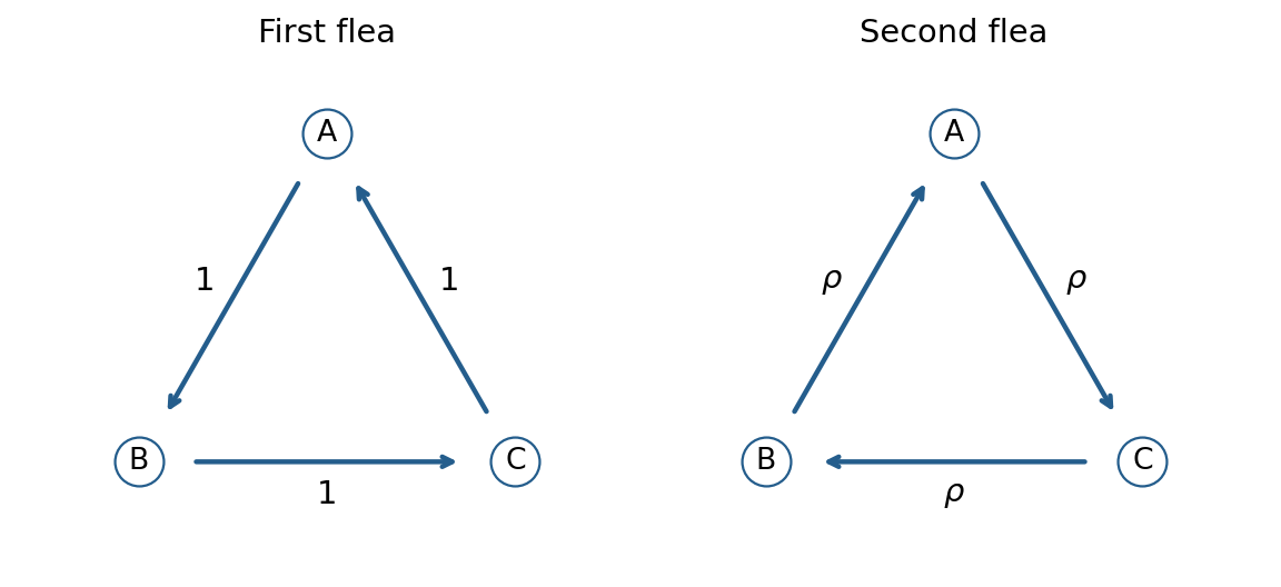
The second continuous-time Markov chain runs in the reverse direction at rate $\rho$, as in the right diagram. Its nonzero eigenvalues have real part $-3\rho /2$, and its transition probabilities tend to $1/3$ for each vertex. Independence therefore givesThus the limit exists for every pair of starting vertices and equals $\boxed{1/3}$.

One can also see the limit directly without spectral multiplication. For fixed starting vertices, $X_t-Y_t$ modulo three advances with each jump of either flea. Its jump count is the sum of independent Poisson processes with rates $1$ and $\rho$, hence is Poisson with rate $1+\rho$ (multiply their generating functions). The formula from part (a), with $t$ replaced by $(1+\rho )t$ and the appropriate initial residue, gives $p(t)$ and the same limit.

Number the vertices $A,B,C$ by $0,1,2$. The continuous-time Markov chain moves one step forward cyclically at rate one, as shown in the left diagram.

Write $P$ for the cyclic shift matrix, so $Q=P-I$. With $\omega =e^{2\pi i/3}$, the eigenvalues of $P$ are $1,\omega ,{\omega }^2$ and those of $Q$ areThe stationary distribution is uniform. A jump count is a rate-one Poisson process, and the displacement is that count modulo three. The roots-of-unity filter $1_{n\equiv d(3)}=\frac{1}{3}{\sum }_{j=0}^2{\omega }^{j(n-d)}$ and $E(s^{N_t})=e^{t(s-1)}$ therefore give, for $d=(y-x)\mathrm{mod}3$,These are also the entries of $e^{tQ}$ obtained by diagonalizing $Q$. In particular,

An isometry preserves the Levi-Civita connection. To justify this, transport the connection on $X$ by $d\psi$. It is torsion-free and preserves the metric on $Y$, since $\psi$ preserves the metric and Lie brackets. These two properties characterize the Levi-Civita connection uniquely: if two such connections differ by $A$, the tensor $a(U,V,W)=⟨A(U,V),W⟩$ is symmetric in its first two arguments and antisymmetric in its last two. Cycling these symmetries yields $a=-a$, hence $A=0$. ThereforeApplying this along $\gamma$ shows that the covariant acceleration of $\psi \circ \gamma$ is zero, so an isometry carries affinely parametrized geodesics to geodesics.

The same identity and the definition $R(U,V)W={\nabla }_U{\nabla }_{V}W-{\nabla }_V{\nabla }_{U}W-{\nabla }_{[U,V]}W$ show that $d\psi$ intertwines the Riemann curvature tensor. If $e_1,e_2$ is an orthonormal tangent basis, its image is orthonormal and

Both proposed converses are false. Take $X=Y={\mathbb{R}}^2$ with the Euclidean metric and $\psi (x)=2x$. A geodesic $p+tv$ maps to the geodesic $2p+2tv$, and both Gaussian curvatures vanish identically. Nevertheless $\psi$ multiplies lengths by two, so is not an isometry. This one counterexample answers both unheaded continuation requests.

A parametrized curve is a geodesic when its covariant acceleration vanishes, ${\nabla }_{\dot{\gamma }}\dot{\gamma }=0$, for the induced Levi-Civita connection. In coordinates this isEquivalently, for an embedded surface its ordinary acceleration is normal to the tangent plane. The parameter is affine; arbitrary reparametrizations need not remain geodesics.

The local existence and uniqueness theorem says that for every $p\in X$ and $v\in T_{p}X$ there is a unique geodesic with $\gamma (0)=p$, $\dot{\gamma }(0)=v$, on a maximal open interval containing zero, depending smoothly on $(p,v)$. This follows from the local existence and uniqueness theorem for the smooth first-order system in $(\gamma ,\dot{\gamma })$. The exponential map is ${\exp }_p(v)={\gamma }_v(1)$ wherever the solution exists through time one. Its domain contains a neighborhood of zero, and $d({\exp }_p{)}_0=I$, since ${\exp }_p(tv)={\gamma }_v(t)$. Thus it is a local diffeomorphism near zero. Completeness is not assumed for a general surface; on a complete surface it is defined on all of $T_{p}X$.

The global Gauss-Bonnet theorem for the induced Riemannian metric isHere $K$ is the Gaussian curvature, $dA$ the induced surface-area element, and $\chi (X)$ the Euler characteristic. For a connected orientable compact surface of genus $g$, $\chi (X)=2-2g$. For several components, sum their contributions. There is no boundary-curvature term because $X$ has no boundary.

The exact condition for this diagonal operator on sequence space isFirst, $T$ is bounded precisely when ${\sup }_n|{\lambda }_n|<\infty$, with operator norm equal to that supremum: the upper bound follows by summing $|{\lambda }_n{x}_n{|}^2$, and the coordinate unit vectors $e_n$ give the lower bound. If the supremum is infinite, choose distinct indices with $|{\lambda }_{n_j}|\ge j$ and set $x_{n_j}=1/j$, other coordinates zero. Then $x\in {\ell }^2$ but $Tx\notin {\ell }^2$, so the displayed prescription would not even define an everywhere-defined map into ${\ell }^2$.

If $T$ is compact but ${\lambda }_n\nrightarrow 0$, infinitely many indices satisfy $|{\lambda }_n|\ge ϵ>0$. Along those indices,contradicting compactness. Conversely, if ${\lambda }_n\to 0$, truncate to $T_{N}x=({\lambda }_1{x}_1,\dots ,{\lambda }_N{x}_N,0,\dots )$. This is a finite-rank compact operator, and $\Vert T-T_N\Vert ={\sup }_{n>N}|{\lambda }_n|\to 0$. To see compactness directly, approximate the image of the unit ball by $T_N$ to within $ϵ/2$, and cover its bounded finite-dimensional image by finitely many $ϵ/2$-balls. Hence $T$'s unit-ball image is totally bounded; its closure is compact because ${\ell }^2$ is complete.

Suppose otherwise and choose linearly independent eigenvectors $v_n$ with $T{v}_n={\lambda }_n{v}_n$ and $|{\lambda }_n|>a$. Put $F_n=\mathrm{span}(v_1,\dots ,v_n)$. Each $F_n$ is finite-dimensional and $T$-invariant. Moreover $(T-{\lambda }_{n}I)F_n\subseteq F_{n-1}$, including when some eigenvalues coincide.

Apply the supplied distance fact inside the Banach space $F_n$ to choose $x_n\in F_n$ with $\Vert x_n\Vert =1$ and $\mathrm{dist}(x_n,F_{n-1})=1$. For $m<n$, both $(T-{\lambda }_{n}I)x_n$ and $T{x}_m$ belong to $F_{n-1}$. ConsequentlyThus $(T{x}_n)$ has no Cauchy subsequence, although $(x_n)$ is bounded. This contradicts the compact operator property. Only finitely many linearly independent eigenvectors can have eigenvalue modulus greater than $a$.

A compact operator is a bounded linear operator carrying every bounded set into a relatively compact set. Equivalently, for every bounded sequence $(x_n)$, the sequence $(T{x}_n)$ has a norm-convergent subsequence. It is enough to require this for the closed unit ball, because any bounded set lies in a scalar multiple of that ball.

For a complex Banach space, the spectrum of a bounded operator and resolvent set areThe bounded inverse theorem says that a bounded bijection between Banach spaces automatically has a bounded inverse, so failure of bijectivity suffices here. The point spectrum isthe set of eigenvalues. For a real Banach space, these definitions use its complexification.

Let $m=[G:H]$, extend $\psi$ to ${\psi }_0$ by zero outside $H$, and choose coset representatives $x_1,\dots ,x_m$. Then $\mathrm{Ind}\psi (g)={\sum }_{j=1}^m{f}_j(g)$ with $f_j(g)={\psi }_0(x_j^{-1}g{x}_j)$. Each summand has squared $G$-normsince $\psi$ is irreducible. Pointwise Cauchy-Schwarz inequality gives $|\sum f_j{|}^2\le m\sum |f_j{|}^2$. After summing and dividing by $|G|$,The $e_i$ are nonnegative integers by part (b). This proves the character induction norm bound without an assumption that $H$ is normal.

The induced character construction extends any class function $\psi$ on $H$ byFrobenius reciprocity for class functions is $⟨{\mathrm{Ind}}_H^G\psi ,\chi {⟩}_G=⟨\psi ,{\mathrm{Res}}_H^G\chi {⟩}_H$. It follows directly by substituting this sum into the left inner product, writing $g=xh{x}^{-1}$, and using the conjugacy invariance of $\chi$. If $\psi$ is a character, its inner product with every restricted irreducible character is a nonnegative integer, a multiplicity in its complete reducible decomposition. Expanding in the orthonormal irreducible-character basis therefore makes $\mathrm{Ind}\psi$ a nonnegative integer sum of irreducible characters: it is a character of $G$.

If $U$ affords $\psi$, a concrete induced representation is $\mathbb{C}[G]{\otimes }_{\mathbb{C}[H]}U$, with $G$ acting by left multiplication on the first factor. Choosing coset representatives decomposes it into $[G:H]$ copies of $U$. An element $g$ permutes these copies; only fixed cosets contribute trace, and the contribution from $xH$ is $\psi (x^{-1}gx)$. Summing fixed cosets gives exactly the displayed induced class function.

The restriction of a representation $\rho :G\to \mathrm{GL}(V)$ to $H$ is the same vector space and operators with the domain limited to $H$; its character is ${\chi }_H(h)=\chi (h)$. Averaging a positive Hermitian inner product over $H$ makes it invariant, so invariant subspaces have invariant orthogonal complements. Repeating gives a direct sum of irreducible $H$-spaces and hence ${\chi }_H={\sum }_i{d}_i{\psi }_i$ with nonnegative integer multiplicities.

By character inner product orthogonality,since $\chi$ is irreducible and has normalized squared norm one on $G$. Equality holds precisely when the omitted nonnegative terms vanish, namely $\boxed{\chi (g)=0\text{ for every }g\notin H}$. This is the restriction multiplicity bound.