
Finite set Created 2026-09-24 Updated 2026-11-05
A finite set is a set admitting a bijection with for some nonnegative integer , including the empty set at . The number is uniquely determined and is its cardinality.
Every injective map from a finite set to itself is surjective, and conversely. This follows by counting image elements: an injection cannot omit an element without reducing the size of its image. For infinite sets the property can fail, as is an injection of the natural numbers into themselves that omits zero. The bijection definition gives a precise meaning to finite without reusing the word in its own definition.
Hermitian form Created 2026-09-24 Updated 2026-10-14
A Hermitian form is a sesquilinear form on a complex vector space satisfying conjugate symmetry,Hence is a real number for every vector. In a basis, the matrix of a Hermitian form has and obeys , equivalently : it is a Hermitian matrix. The coordinate rule remains . Conjugate symmetry does not imply positivity.[ref]
https://sites.math.washington.edu/~burke/crs/554/lectures/b-lecture4.pdf. Burke, Linear Analysis, Lecture 4, Hermitian symmetry
The diagonal contains more information than might be expected. For any complex sesquilinear form , put . Expanding four expressions gives the complex polarization identity in the linear-first convention:This is an algebraic identity, with no positivity assumption. If every is real, interchanging preserves the first difference and negates the second: use for . The identity then gives . Thus a complex sesquilinear form is a Hermitian form if and only if all its diagonal values are real. Testing only the basis vectors is insufficient: the off-diagonal example in sesquilinear form has zero diagonal entries in its matrix but a nonreal value at .
Consider the indefinite Hermitian formIts values at are . Moreover and are nonzero isotropic vectors: , yet . These vectors do not belong to the radical of a Hermitian form, and the usual Cauchy-Schwarz inequality would incorrectly require . An indefinite Hermitian form records signed geometry rather than defining a norm by .
There is a separate boundary case: is a positive semidefinite Hermitian form, since , but . Its radical of a Hermitian form is the entire second coordinate line. Positive definiteness is exactly the additional condition in a Hermitian inner product. The three examples below show why these distinctions matter: on the real slice , has an ellipse as its unit level, has hyperbolas, and has two parallel lines. These are slices of the complex examples, not drawings of their full four-dimensional domains.
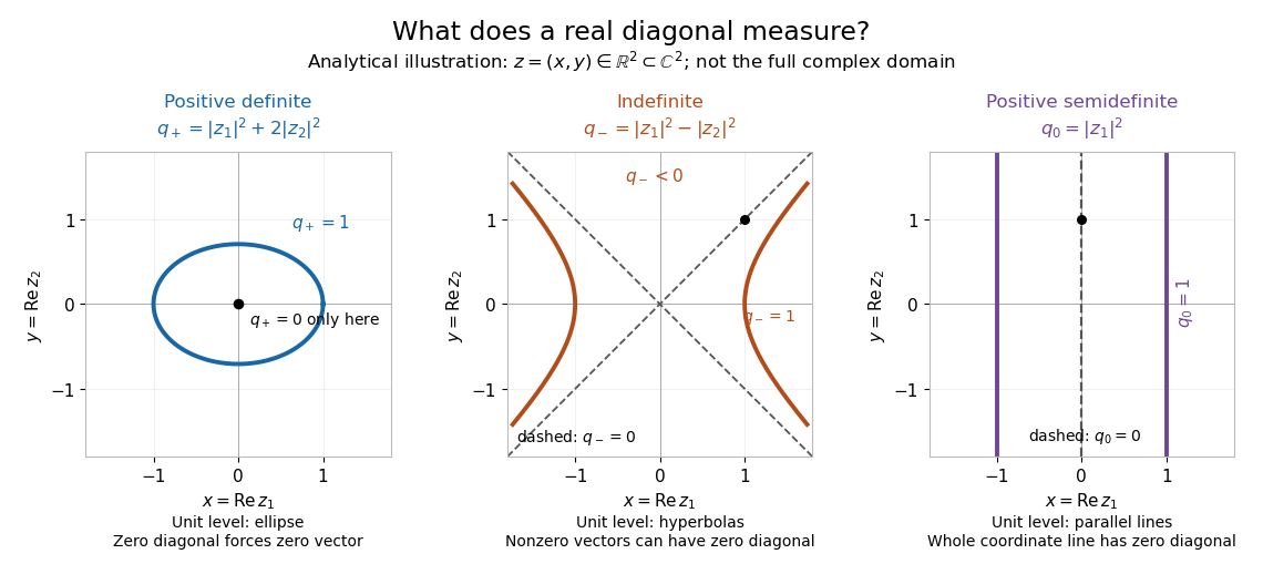
Analytical illustration: real slices of positive definite, indefinite, and positive semidefinite Hermitian forms
. Details. Hydrogen ground-state energy Created 2026-09-24 Updated 2026-09-24
Uniform limit Created 2026-09-24 Updated 2026-11-05
A function is the uniform limit of a sequence of functions whenEquivalently the supremum error tends to zero. The same index works for all inputs, including inputs chosen differently for each . A uniform limit of continuous functions is continuous, by approximating both endpoint values with one common approximant.
For on , , the zero function is a uniform limit because the supremum error is . On , the pointwise limit instead equals zero below one and one at one. Its supremum error remains one for every , so there is no uniform limit there. The open supremum below the endpoint need not be attained to obstruct uniform convergence.
Convergent series Created 2026-09-24 Updated 2026-10-14
Asymptotic equivalence Created 2026-09-24 Updated 2026-10-14
For functions with nonzero sufficiently near a specified limit,The same definition applies to sequences as . Equivalently, : replacing by has a relative error tending to zero, and the difference is in little o notation. The limit and reference scale are essential parts of the statement.
For example, because . Replacing the former by the latter gives absolute error , which grows without bound. Thus asymptotic equivalence controls a ratio, rather than requiring the absolute error to vanish. This distinction is crucial when approximating a rapidly growing factorial with Stirling's formula.
By contrast, and have the same order in big theta notation, but are not asymptotically equivalent: their ratio remains two. For positive functions, asymptotic equivalence gives both-sided constant bounds eventually, whereas constant bounds alone do not recover the leading coefficient.
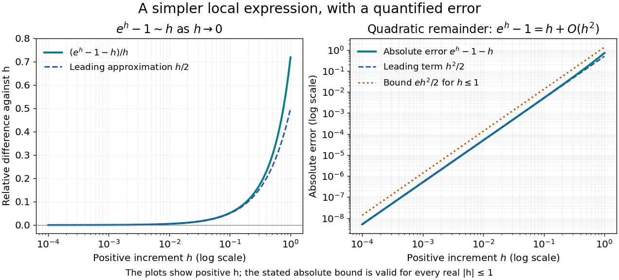


For a local example with real , the exponential function obeys as . The Taylor theorem with Lagrange remainder givesThus for ,This states in big O notation, and division by shows that the relative difference measured against vanishes. The diagram uses positive ; the bound is valid on both sides of zero. At , the absolute error is approximately and the relative difference against is approximately .
Harmonic sum Created 2026-09-24 Updated 2026-10-03
Total variation Created 2026-09-24 Updated 2026-11-05
Total variation measures accumulated absolute change rather than just the difference between two endpoint values. For a real or complex sequence , its total variation isallowing . The triangle inequality gives . Finite variation therefore makes the sequence Cauchy and hence convergent in or .
The converse fails. The sequence tends to zero, but , whose sum diverges. Small late values can still accumulate infinitely much back-and-forth movement.
For a function on an interval, the total variation of a function replaces the sum over consecutive indices by a supremum over all partitions of an interval. For spatial fields, the total variation seminorm on a domain uses the distributional derivative as a measure. Total generalized variation extends that regularization idea to higher-order structure. These settings share cumulative-change control, while their definitions specify different index or spatial domains.
Absolute convergence Created 2026-09-24 Updated 2026-10-14
A series converges absolutely when the series of absolute values converges; absolute convergence implies convergence.
P-series Created 2026-09-24 Updated 2026-10-03
Conditional convergence Created 2026-09-24 Updated 2026-09-24
Cauchy sequence Created 2026-09-24 Updated 2026-10-14
A Cauchy sequence is a sequence whose sufficiently late terms are all close to one another. In a metric space , the precise condition isFor real numbers with their usual metric, . The useful feature is that the definition compares computed terms to other computed terms: it does not require an already known limit of a sequence. The one index must control every pair of later indices, not merely successive terms. [ref]
https://www.jirka.org/ra/html/sec_cauchy.html. Lebl, Basic Analysis I, §2.4: Cauchy sequences and the role of all late pairs
.For an explicit example, take for . Its tail of a sequence beginning at lies in , and for every ,Choose with to certify the entire future sequence. For , works because . The limit of a sequence is one, but the pairwise bound establishes the Cauchy sequence property without first needing that answer. By contrast, is not a Cauchy sequence: arbitrarily late even integers and odd integers give values separated by two. [ref]
https://www.ocw.mit.edu/courses/18-100a-real-analysis-fall-2020/mit18_100af20_lec102.pdf. MIT 18.100A, Lecture 10, Definition 1, Negation 3 and Example 4
.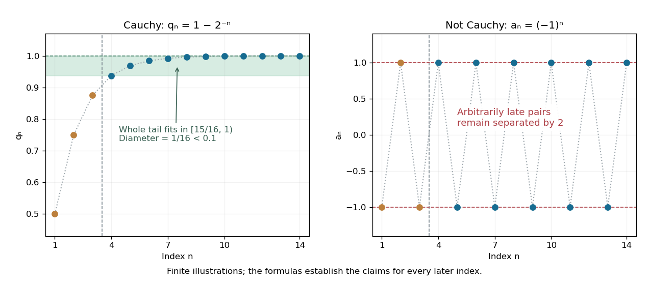
A Cauchy sequence confines every sufficiently late pair to a small band; persistent alternation cannot do so
. The original geometric example has all terms with in , a band narrower than . Only finitely many terms are drawn; the formula certifies the entire tail. The alternating example continues to attain both and arbitrarily late. Details.
Tiny successive changes do not provide this guarantee. For the harmonic numbers , the successive difference tends to zero, butThus, beyond every proposed , choosing and defeats the fixed tolerance . Even every fixed positive lag passes the weaker test: . The failing lag grows with , as explained more generally by convergence from arbitrary variable-lag increments. [ref]
https://www.jirka.org/ra/html/sec_cauchy.html. Lebl, Basic Analysis I, §2.4: shrinking fixed-lag increments do not imply the Cauchy condition
.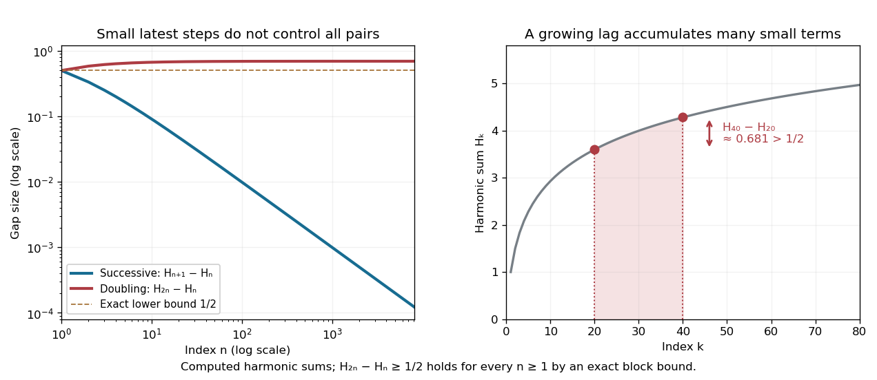
Harmonic numbers take vanishing successive steps while retaining a nonvanishing gap between indices and
. The blue curve is ; the red curve is . The exact lower bound holds for every positive integer , not just the plotted sample. The shaded region between and in the right panel illustrates how many individually small terms produce a substantial gap. Details.
Every convergent sequence in a metric space is a Cauchy sequence: apply the triangle inequality to two late terms and their common limit of a sequence. The reverse implication requires completeness. It holds in the real numbers by completeness of the real numbers, but can fail in the rational numbers: the rational endpoints from the bisection method approaching are a Cauchy sequence with no rational limit of a sequence. The existing construction in completeness of the real numbers shows how this happens. A Cauchy sequence is always a bounded sequence; in , boundedness gives a convergent subsequence by the Bolzano-Weierstrass theorem, and the pairwise condition forces the whole sequence to share its limit. [ref]
https://www.ocw.mit.edu/courses/18-100a-real-analysis-fall-2020/mit18_100af20_lec102.pdf. MIT 18.100A, Lecture 10, Theorems 5–7: boundedness, subsequences and real completeness
. Geometric series Created 2026-09-24 Updated 2026-10-20
A geometric series adds the terms of a geometric progression:Its ordinary infinite sum is the limit of a sequence of partial sums , rather than a new operation that adds infinitely many terms at once. For that are real numbers or complex numbers, if , the series is absolutely convergent andWhen , this condition on the modulus of is also necessary: for the terms fail to tend to zero. The all-zero series converges for every . The finite geometric series identity and give the result with almost no extra algebra. [ref]
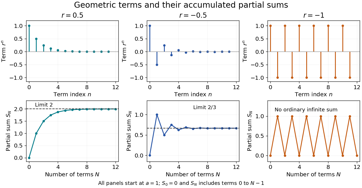
Decaying terms, accumulating sums, and the failure of an undamped alternating series
. Details. 
With and , the partial sums approach from below. Changing the common ratio to makes the partial sums approach from alternating sides: their increments still shrink. At , those increments never shrink, and the partial sums remain . Substituting into does not supply the ordinary sum of that divergent series.
The formula is useful because many apparently different problems share a fixed multiplier. A repeating decimal such as isA geometric distribution counting failures before the first success normalizes by the same identity: for , the probabilities on add to one. The comparison test for series uses a bound by a decaying geometric progression to establish absolute convergence without an exact formula for the series being studied. The iterated contraction gives a summable orbit result uses precisely this idea for repeated applications of a map.
The remainder of a geometric series gives more than an eventual limit: it states exactly how much an approximation omits. A common ratio close to one still gives a convergent series, but can require many terms for a useful approximation.
Uniform convergence Created 2026-09-24 Updated 2026-10-14
A sequence of functions converges uniformly to , where is a metric space with metric , precisely whenFor real numbers, use the absolute value . Compare the universal quantification and existential quantification:The decisive change is whether can depend on . Uniform convergence implies pointwise convergence.[ref]
6.1 Pointwise and uniform convergence. Basic Analysis: Introduction to Real Analysis, Volume I by Jiří Lebl, §6.1.2, Definition 6.1.6 and Proposition 6.1.7
For functions taking values in real numbers on a nonempty domain of a function, the supremum error is , allowing . Then uniform convergence is equivalent to . The supremum need not be a maximum: pointwise strict bounds below only give , so use tolerance when proving this equivalence. This single error bound controls every possible input, including one chosen after seeing the index.
For and its pointwise limit on , the error is zero at one but approaches one as from below. Consequentlyfor every positive integer . This supremum is never attained: below one the error is , and at one it is zero. Deleting the endpoint leaves the same supremum error on . To disprove uniform convergence directly, choose : for any proposed , take and . The error equals , violating the strict tolerance. Thus a moving input defeats every proposed common threshold.
On the smaller interval , for a fixed , the pointwise limit is zero andFor and , the exact first successful common threshold isThe logarithm and floor function turn an infinite approximation statement into a finite stopping rule. At , fails tolerance , while succeeds. At and , the ratio is exactly three: is necessary because equality is insufficient. For , every error is zero. The domain of a function determines whether one threshold can certify every input.
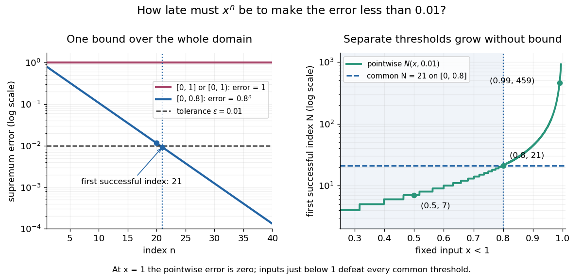

For another explicit stopping rule, let on . Its uniform limit is zero and its supremum error is . For every , works, using the ceiling function. Unlike on , it controls even the endpoint.
The practical beauty of uniform convergence is that one quantitative bound can survive further operations: the uniform limit theorem preserves continuity, and uniform convergence preserves integrals on a compact interval controls accumulated error. Differentiation needs additional hypotheses, such as uniform derivative convergence with an anchored value. These results distinguish an approximation that looks accurate at selected inputs from one that justifies replacing a whole function in a calculation.
Power series Created 2026-09-24 Updated 2026-10-14
A power series combines a sequence of coefficients with monomials in the displacement from a fixed centre:The variable , centre , and coefficients can be real numbers or complex numbers. Its degree- partial sum is a polynomial, so a convergent power series can turn a complicated function into increasingly accurate finite calculations. Convergence, and the error after stopping, are essential parts of that claim.
The geometric series supplies the simplest computed example:At , stopping after degree ten gives , differing from the exact value by . At , the same degree gives only about instead of . The same formula has very different practical accuracy at different points; the geometric power-series remainder quantifies it.
The structure is useful beyond numerical evaluation. Within its radius of convergence, termwise differentiation of a power series turns a question about a derivative into a question about coefficients. A Taylor series chooses when it represents the function locally. A formal power series instead uses the coefficients algebraically, without asserting numerical convergence; the existing generating function examples use that distinction to encode counting problems.
Pointwise convergence Created 2026-09-24 Updated 2026-10-14
For a sequence of functions , pointwise convergence to a function meansIt is the ordinary limit of a sequence at each fixed input. The threshold may depend on the input. Uniform convergence instead requires one threshold for the entire domain of a function.[ref]
6.1 Pointwise and uniform convergence. Basic Analysis: Introduction to Real Analysis, Volume I by Jiří Lebl, §6.1.1, Definition 6.1.1 and Proposition 6.1.5
Consider the polynomial functions , for positive integers , on the interval . For the geometric sequence tends to zero, while . ThusEach is a continuous function, but its pointwise limit is discontinuous at one. Holding an input still hides what happens near that endpoint. The analogous even-power example on appears in the source.[ref]
For and , taking the logarithm of and dividing by the negative real number reverses the inequality:The floor function followed by adding one handles the strict inequality even when the ratio is an integer. For tolerance , the first successful indices at , , and are respectively , , and . At , fails and succeeds. At and , the error from this pointwise limit is already zero, so works. Nevertheless, grows without bound as from below. A finite list of accurate test inputs cannot establish uniform convergence.
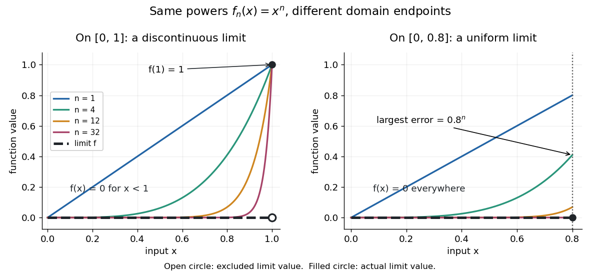

An even sharper warning concerns integration. On , define the continuous functionsTheir supports are , with height at and value zero at both ends. Every fixed eventually lies beyond the support, and always, so pointwise convergence gives the zero function. Nevertheless, each integral is the area of a triangle: . Shrinking width compensates increasing height. Hence the limit of a sequence of these integrals differs from the integral of the pointwise limit; interchanging them requires additional conditions, such as uniform convergence preserves integrals on a compact interval.
Fibonacci number Created 2026-09-24 Updated 2026-10-20
Convergent sequence Created 2026-09-24 Updated 2026-11-05
A real sequence is convergent if there exists a real number such that, for every , some index satisfies whenever . The same definition uses a metric in a metric space; a general topological space uses eventual membership in every neighborhood of the limit.
For , choose to prove convergence to zero. For , even and odd subsequences have different limits, so no real limit exists. Convergence depends on the ambient space: rational approximations to converge in the real numbers but have no limit within the rational numbers.
Bolzano-Weierstrass theorem Created 2026-09-24 Updated 2026-10-14
Every bounded sequence of real numbers contains a subsequence with a finite limit of a sequence. If for every positive integer , there are integers and a real number such thatThe increasing indices matter: a subsequence retains the original order and selects terms arbitrarily far along the original sequence. The theorem guarantees the existence of at least one such selection; it does not claim that the entire sequence converges or that the subsequential limit is unique.[ref]
For example, the bounded sequence has two distinct subsequential limits:The even terms form a convergent sequence, and so do the odd terms. The full sequence cannot have a limit of a sequence because its two subsequences have different limits. Its limit superior is and its limit inferior is .
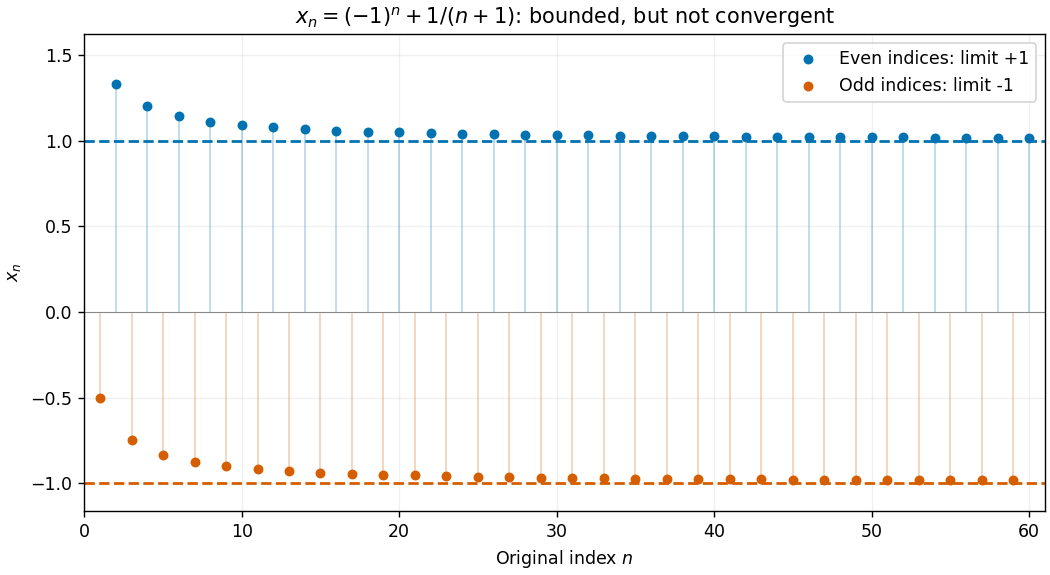

This is useful when a construction produces many candidate points but does not immediately produce a convergent sequence. For a continuous function on a nonempty closed bounded feasible region in a finite-dimensional Euclidean space, take a sequence whose objective values approach the infimum. A convergent subsequence supplies a candidate point; a closed subset retains that point, and continuity passes the objective values to the limit of a sequence. This is the mechanism behind attainment in the extreme value theorem. The diagonal subsequence argument extends the real-sequence theorem to finite-dimensional Euclidean space.
There are unlisted articles, also show them or only show them.