
Slice knot Created 2026-09-24 Updated 2026-09-24
Seifert surface Created 2026-09-24 Updated 2026-09-24
A Seifert surface for an oriented knot is a compact connected oriented surface with oriented boundary .
Satellite knot Created 2026-09-24 Updated 2026-09-24
A satellite knot is obtained by embedding a patterned solid torus into a tubular neighborhood of a companion knot .
Torus knot Created 2026-09-24 Updated 2026-10-14
For nonzero coprime integers , the torus knot lies on a standard unknotted torus in the three-sphere and winds times meridionally and times longitudinally. Here a meridian of a solid torus goes around the small cross-section of the doughnut, while the longitudinal direction goes around its central hole. The integers count signed turns, so changing one sign gives the mirror of a link of the torus knot. In this article is always the meridional count and the longitudinal count.
An explicit parametric curve in three-dimensional Euclidean space iswhere . Its cylindrical radius satisfies , the equation of the supporting torus. Its meridional angle is and its longitudinal angle is : this checks the convention directly rather than relying on the picture. Its squared speed isIf two parameter values give the same point, their difference satisfies . Bézout's identity for the coprime integers then gives . Thus the loop closes and is an injective function on the parameter circle, with nonzero derivative; it is a smooth embedding.
For example, , , , produces a trefoil knot. During one circuit the meridional angle changes by and the longitudinal angle by . The supporting torus is a guide for construction, not a constraint on later ambient isotopies: the knot may move off it. This family makes arithmetic visible as geometry: the coprime integers determine whether a single traversal visits the whole loop without repetition.
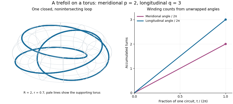

The coprime integers hypothesis matters. If the greatest common divisor is , the same parametric curve retraces a single component times; it does not automatically draw different components. The corresponding torus link is instead the full set of points on the torus whose angles satisfy , with meridional angle and longitudinal angle . It has disjoint components, each with winding counts . For instance, the torus link consists of two parallel loops and is a Hopf link, whereas substituting into simply traces one of those loops twice.
Connected sum of knots Created 2026-09-24 Updated 2026-10-14
The connected sum removes a short unknotted arc from each of two oriented knots and joins the four endpoints by an orientation-compatible pair of arcs.
Unknot Created 2026-09-24 Updated 2026-10-14
The unknot is the knot type represented by the planar circleEquivalently, an unknot is a knot that bounds a smoothly embedded disk in the three-sphere. The disk must itself be embedded; merely filling a loop with a map that is allowed to intersect itself does not establish that the knot is an unknot. Flattening a neighborhood of an embedded spanning disk explains why this criterion recovers the planar circle.
A complicated drawing can still represent an unknot. Starting with a crossing-free knot diagram of , insert a small kink by a type I Reidemeister move. The resulting knot diagram has one crossing, but removing the kink exhibits the same unknot. Repeating in separate small regions gives knot diagrams of the unknot with arbitrarily many crossings, although the crossing number of a knot is . A drawing's apparent complexity is therefore not a certificate of knotting.
The normalized Alexander polynomial of a knot and Jones polynomial of the unknot are both , and its knot group is the infinite cyclic group , because the knot exterior is a solid torus. These are useful comparison values. In particular, a nonconstant Alexander polynomial of a knot certifies that a knot is not an unknot, but the converse fails: nontrivial untwisted Whitehead doubles also have Alexander polynomial of a knot .
Oriented knot Created 2026-09-24 Updated 2026-10-03
Dissipation estimate for high-Reynolds-number bubble drag Created 2026-09-24 Updated 2026-11-05
For a clean bubble of size and speed at large Reynolds number, the outer potential flow violates the stress-free condition by a strain of order . A boundary layer of thickness needs a velocity correction only of order , so its dissipation is smaller than the outer-flow dissipation by order . The leading drag power is therefore obtained from
Rotational kinetic energy Created 2026-09-24 Updated 2026-10-14
Rotational kinetic energy is the kinetic energy of a rigid body's rotation. For pure rotation about an axis fixed in an inertial frame,Here is the perpendicular distance of a mass element from that axis, is the moment of inertia about that same axis, and is the common angular speed, measured in radians per second. The rigid body assumption fixes the relative positions of the mass elements; they share angular velocity but have different speeds . Summing their kinetic energies gives the formula. This is a nonrelativistic model; deformation or internal motion can contribute additional kinetic energy.[ref]
For a computed example, take a uniform disc and an ideal thin ring, each of mass and radius , rotating about its central perpendicular axis at angular speed . The moment of inertia of a uniform disc is , while the ring has moment of inertia . Their rotational kinetic energies are therefore and . The ring stores twice the energy at the same angular speed, because more mass lies farther from the axis. At the same nonzero rotational kinetic energy, its angular speed would instead be times the disc's. This makes radial placement useful for storing energy in a rotating wheel, although a real design must also withstand the stresses of rotation.
For fixed-axis rotation with constant moment of inertia, write the signed rotation rate as , with angle in radians. The axial component of net external torque obeys , so the work-energy theorem becomesAn opposing torque removes rotational kinetic energy; bearing friction must be included in the net torque. The signed matters when the direction reverses. Rotation about a fixed axis need not be about a principal axis: the scalar energy formula still holds, but transverse bearing torques can be needed to maintain that axis.
For general rigid body motion, use the inertia tensor about the centre of mass :This is the kinetic-energy decomposition about the centre of mass. In a principal body frame, the rotational term is , using the principal moments of inertia. Away from a principal axis, angular momentum and angular velocity need not be parallel. A freely rotating asymmetric rigid body can change the direction of angular velocity relative to the body even while rotational kinetic energy remains constant; Euler equations for a torque-free rigid body govern that motion. One constant axial moment of inertia is then insufficient.[ref]
Kerr polar tortoise coordinate Created 2026-09-24 Updated 2026-09-24
Kerr ergoregion Created 2026-09-24 Updated 2026-11-05
For a Kerr black hole, let be the stationary Killing vector field normalized at infinity. The exterior Kerr ergoregion is where , so the tangent to motion following alone would be a spacelike vector. A physical observer there cannot remain at fixed angular coordinates relative to infinity.
For nonzero spin its outer stationary-limit surface isIt lies outside the outer event horizon except where they meet on the rotation axis. A causal curve can escape this exterior Kerr ergoregion; forced co-rotation does not make it the black-hole interior. The conserved Killing energy can be negative there, enabling the Penrose process, while locally measured future-particle energy remains positive.[ref][ref]
Boyer-Lindquist coordinates Created 2026-09-24 Updated 2026-10-06
Boyer-Lindquist coordinates adapt the Kerr metric to its stationary and axial symmetries. The horizon radii are the roots of .
Rank-nullity theorem Created 2026-09-24 Updated 2026-10-14
The rank-nullity theorem accounts for the input dimensions of a linear map: the number of independent invisible input directions plus the number of independent reachable output directions equals the input dimension. For over a field, with finite-dimensional domain of a function ,Here is the nullity, and is the rank of a linear map. The kernel lives in the input vector space, while the image of a linear map lives in the output vector space. For an -by- matrix of matrix rank , the formula is : the number of columns counts input coordinates. [ref]
Linear Algebra Done Right by Sheldon Axler (4th edition). Sheldon Axler, Linear Algebra Done Right, fourth edition, §3B: fundamental theorem of linear maps
For a computed example over the real numbers, takeThe kernel is and the image of a linear map is . Each has dimension one, so the two input dimensions split as . The vector can be writtenThe second summand is undetectable: . The picture uses the standard dot product to choose a visible direction perpendicular to the kernel; this is a convenient geometric choice, not an extra hypothesis of the rank-nullity theorem.
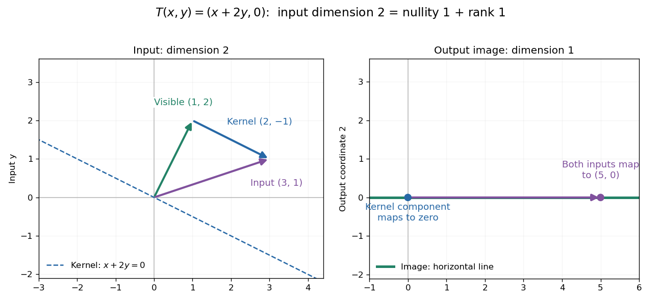
Two input dimensions split into one visible direction and one kernel direction
. For , the input splits into and . Both and map to , while the kernel component maps to zero. The horizontal output line is the entire image of a linear map. Details.
This explains a practical tradeoff in a linear system. If , every other input with output is for . The nullity therefore counts independent freedom in an existing solution; the rank counts independent reachable output directions. In the example, has all solutions , while has none. The cokernel records this failure of reachability.
For an -by- matrix, injectivity requires matrix rank , and surjectivity requires matrix rank . When , these conditions differ. For example, with has rank one and nullity two, because . The input accounting is , although only one of two output directions is reached.
Proof outline: extend a basis of the kernel to a basis of . Every output is a linear combination of because the vanish under . If a linear combination of the is zero, the corresponding combination of the lies in the kernel; linear independence of the full basis forces all its coefficients to vanish. Thus the added basis vectors give a basis of the image of a linear map. Counting them proves the formula.
Circular Kepler orbit Created 2026-09-24 Updated 2026-09-24
Specific angular momentum Created 2026-09-24 Updated 2026-09-24
The specific angular momentum is angular momentum per unit mass, . For a planar Kepler orbit its magnitude is .
Specific orbital energy Created 2026-09-24 Updated 2026-11-05
The specific orbital energy is the relative mechanical energy per unit reduced mass in the Newtonian two-body problem. For total mass , gravitational parameter , separation and relative speed , it isThe gravitational potential is taken to vanish at infinite separation. The last equality uses a signed semi-major axis : positive for a bound ellipse and negative for a hyperbolic Kepler orbit. A parabolic Kepler orbit has and no finite semi-major axis. For nonradial attractive Kepler orbits, these signs distinguish the three orbit classes.[ref]
For a circular orbit, gives . For an escaping hyperbolic Kepler orbit, taking gives the hyperbolic excess speed . Multiplication by the reduced mass gives the two-body orbital energy; dividing by a different mass would mix conventions. The units of specific orbital energy are .
Orbital element Created 2026-09-24 Updated 2026-09-24
An orbital element is one of a set of parameters specifying an orbit at a chosen epoch. For a Kepler orbit, the semi-major axis and eccentricity determine its size and shape, while angular elements determine its orientation and the body's position.
Semi-minor axis Created 2026-09-24 Updated 2026-10-14
Semi-major axis Created 2026-09-24 Updated 2026-10-14
Apoapsis Created 2026-09-24 Updated 2026-10-07
There are unlisted articles, also show them or only show them.