
Euclidean algorithm Created 2026-09-24 Updated 2026-11-05
For positive integers , the Euclidean algorithm repeatedly performs division with remainder: write with , then replace by until the second entry is zero. The final nonzero entry is their greatest common divisor. A remainder preserves the set of common divisors: an integer divides and exactly when it divides and . The positive remainders strictly decrease, so the calculation terminates.
The complete calculation for and isHence . The fraction reduces to by dividing numerator and denominator by that common factor. The same remainder calculation has a geometric interpretation: remove squares from a -by- rectangle, then repeat on the remaining strip. Each division step records how many equal squares fit and the width of the new strip.
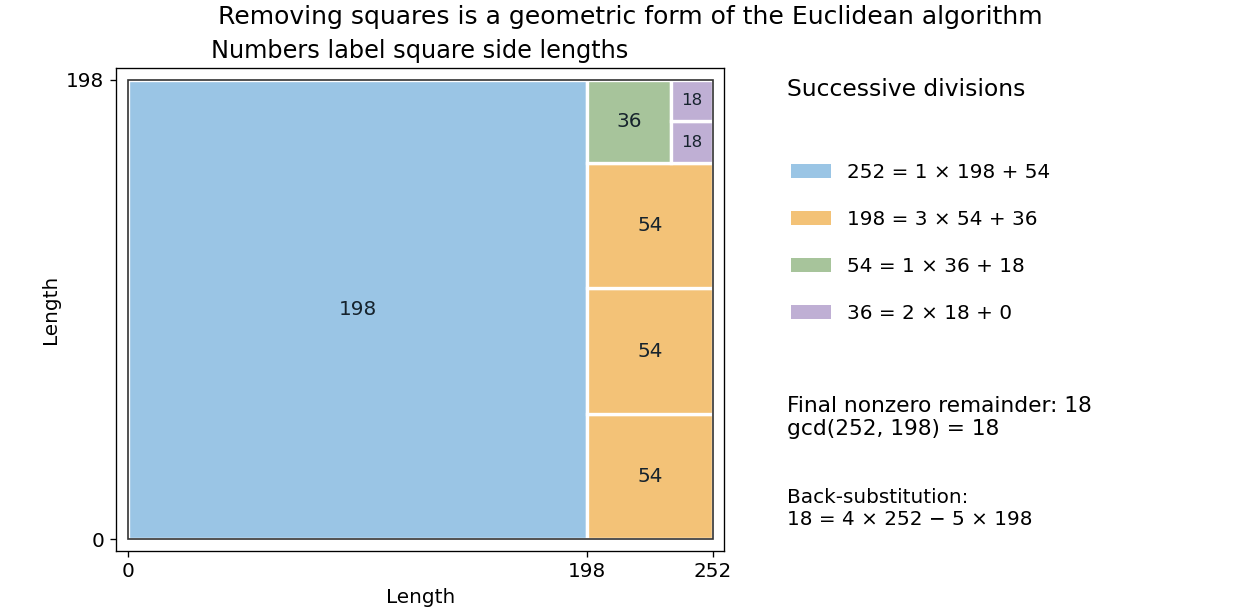
Successive square removals record the Euclidean algorithm for 252 and 198
. Details. The procedure does more than test individual divisors. Each step replaces the whole common-divisor problem by a smaller equivalent one. Euclid's Book VII, Proposition 2 describes the corresponding repeated-subtraction construction; batching those subtractions into division with remainder gives the present formulation. [ref]
https://mathcs.clarku.edu/~djoyce/java/elements/bookVII/propVII2.html. Euclid, Elements VII.2, greatest common measure
Multiplicative order Created 2026-09-24 Updated 2026-10-13
For coprime integers with , the multiplicative order is the least positive integer such thatIt counts the distinct powers in the cyclic subgroup generated by the congruence class of . Thus it is an order of a group element in the unit group .[ref]
A Computational Introduction to Number Theory and Algebra by Victor Shoup. pp. 153 and 156–157, Theorem 6.29
For example, the modular exponentiation , starting at , produces . The first return to one takes three steps, so . Starting at the congruence class three and repeatedly multiplying by two instead gives : these are the other three units modulo seven, outside the cyclic subgroup generated by two.
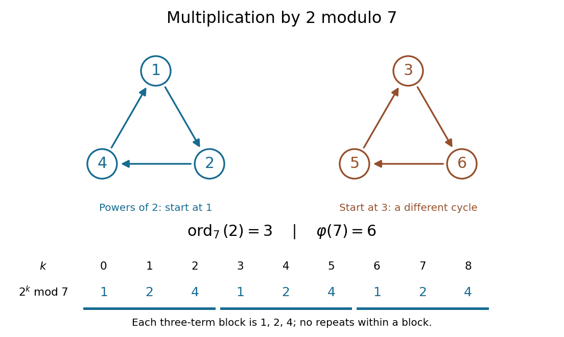
Euler's theorem guarantees a return to one at exponent , where is Euler's totient function. Thus the multiplicative order exists for every unit.[ref]
Euler’s Theorem by Keith Conrad. p. 1, Theorem 1.2; pp. 2–3, permutation of the units and cancellation
In fact,By Lagrange's theorem, the size of the cyclic subgroup divides the size of the unit group, which is Euler's totient function. For two modulo seven, this is ; the multiplicative order need not equal Euler's totient function. If , its multiplicative order is one.The coprime integers hypothesis is necessary: if , any common divisor of and divides one. For instance, powers of two modulo eight give , with no positive-exponent return to one. This sequence eventually settles, but two has no multiplicative order modulo eight.
Carmichael function Created 2026-09-24 Updated 2026-10-20
For an integer , the Carmichael function is the exponent of a finite group for the unit group : the least positive integer for whichHere the greatest common divisor condition selects the units. Euler's totient function counts them; the Carmichael function gives their least common return exponent.[ref]
Modulo eight, the units are , and their squares are all congruent to one. Their multiplicative orders are , so although . Modulo fifteen, the units have multiplicative orders . For example, the powers of two return through . Thus although ; the multiplicative order of four is only two.
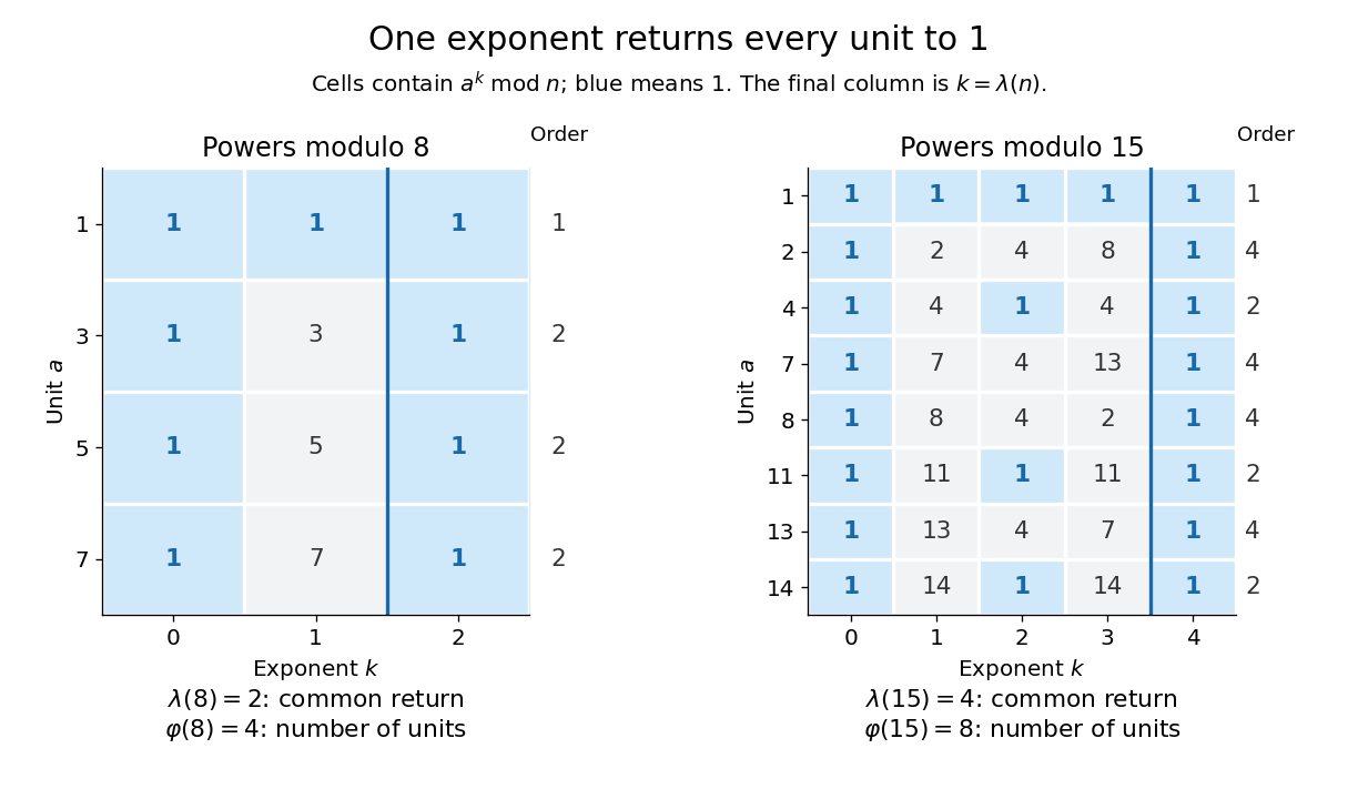


The three quantities are related byA common return exponent must be a multiple of every multiplicative order, hence of their least common multiple. Conversely, that least common multiple makes every unit return to one. Lagrange's theorem makes each multiplicative order divide the group order , proving the final divisibility. The Carmichael function applies to all units at once, while the multiplicative order concerns a chosen unit.
For the prime factorization with distinct prime numbers and , the formulas areThese are least common multiples, rather than products: . The convention handles the trivial case separately.[ref]
The Chinese remainder theorem for unit groups explains the least common multiple: a power returns to one in every prime power component exactly when it is a multiple of each component's exponent of a finite group. For an odd prime power, the unit group is a cyclic group of group order . For , the unit group modulo is a direct product of groups , generated by the classes of and five, so its exponent of a finite group is .[ref]
A Computational Introduction to Number Theory and Algebra by Victor Shoup. Section 7.5, pp. 203–205, Theorem 7.28 and its proof
This gives a uniform reduction for modular exponentiation: for a unit and a nonnegative integer , reduce modulo . For example, because . The unit hypothesis matters: , but . Computing the formula assumes the prime factorization is available. The same common-exponent viewpoint explains Carmichael numbers: a composite number passes the Fermat primality test for every unit base exactly when . For example, .
Rational number Created 2026-09-24 Updated 2026-11-05
A rational number is a quotient of integers with . The numerator can be negative or zero; the denominator can be chosen positive by transferring its sign to . For example, and .
Different fractions describe the same rational number exactly when cross multiplication gives . Dividing the entries by their greatest common divisor produces the unique reduced fraction with positive denominator, including for zero.
The rational numbers form a field: addition, subtraction, multiplication and division by a nonzero rational number remain rational. They are dense in the real line, by density of the rational numbers, although they do not fill it: the square root of two is an irrational number.
Difference of two squares Created 2026-09-24 Updated 2026-11-05
The difference of two squares identity isIt follows by expanding the right side and cancelling its cross terms. It holds for real numbers and, more generally, in a commutative ring.
For integers , the factors and have the same parity. Conversely, any integer factorization with factors of the same parity yields and . Thus an integer is a difference of two squares exactly when it is not congruent to two modulo four: odd values use , and multiples of four use . This is the factor-pair interpretation behind Fermat's factorization method.
Square factor Created 2026-09-24 Updated 2026-11-05
A square factor of an integer is a positive perfect square dividing . Every integer has the trivial square factor one; usually the useful question is whether a nontrivial one, with , occurs.
A positive integer has a nontrivial square factor if and only if some prime number satisfies . One direction takes ; for the other, choose any prime factor of . Equivalently, some prime exponent in is at least two. For example, twelve has square factor four and eighteen has square factor nine, whereas thirty has none other than one. A positive integer without a nontrivial square factor is a square-free integer.
Fermat little theorem Created 2026-09-24 Updated 2026-10-14
For a prime number and an integer not divisible by , Fermat's little theorem states the modular congruenceEquivalently, for every integer , including and multiples of ,The first formulation follows from the second by multiplying by a modular multiplicative inverse of . Conversely, multiply the first by when ; when , both sides of the second are zero modulo . The divisibility condition in the first formulation is essential.[ref]
For , , so and . Also , while : a zero residue class cannot satisfy the first formulation. It does satisfy . A failure at a zero residue class therefore says nothing against a candidate's being a prime number.
The prime number is included. Its only nonzero residue class is one: every odd integer satisfies . Every integer also satisfies , because is even. Testing the first formulation with an even integer would violate its hypothesis.
The useful surprise is that every nonzero residue class returns to one at the same exponent , although its shortest return can be earlier. This gives exponent reduction for units: for a nonnegative integer , when . It also computes a modular multiplicative inverse as modulo , including . Repeated squaring makes these modular exponentiations practical.
In group theory, the nonzero residue classes form the multiplicative group of integers modulo n with , of group order . Lagrange's theorem says that the multiplicative order of divides , giving the guaranteed return. Euler's theorem extends this to a general integer modulus , using the units and Euler's totient function ; the Carmichael function gives the least common return exponent for all units. A nonzero residue class modulo a composite number need not be a unit.
Leonhard Euler's paper presented in 1732 and published in 1738 states a historical formulation: Theorem 1 says that powers with exponent leave zero or one upon division by a prime number . The preceding discussion states the difference-of-powers version and explicitly says that he does not have its proof.[ref]
Euler totient function Created 2026-09-24 Updated 2026-11-05
Euler's totient function is the arithmetic functionIt counts the congruence classes modulo represented by integers coprime to . In particular, , since . For , the coprime integers among are , so ; they form a reduced residue system. [ref]
Floor and arithmetic functions by Darij Grinberg. Darij Grinberg, MIT 18.781 lecture notes, Definition 2.1.2
Counting these congruence classes is useful because they are exactly the classes with modular multiplicative inverses. Their number supplies the exponent in Euler theorem. Möbius inversion gives the product formulawhere runs over distinct prime factors of . Thus for prime powers with , and . The product for is an empty product, so it gives the same convention .
Prime valuation Created 2026-09-24 Updated 2026-10-13
For a prime number and a positive integer , the prime valuation is the exponent of in the prime factorization of , equivalentlyThus because divides but does not; , and . In particular . Multiplication adds prime valuations, , and the fundamental theorem of arithmetic makes comparison of prime valuations an exact test for divisibility between positive integers. This definition extends to a nonzero integer by taking its absolute value; for zero one commonly sets .
Binary quadratic form Created 2026-09-24 Updated 2026-11-05
A binary quadratic form is a quadratic form in two variables, written or . In number theory an integral binary quadratic form has integer polynomial coefficients . It represents an integer when for some integers .
The homogeneous polynomial identity distinguishes a form from a general quadratic polynomial with constant or linear terms. The discriminant of a binary quadratic form is . For example, has and represents , while has and represents at .
Changing integer coordinates can conceal the same arithmetic. Substituting into gives . The transformation has determinant one and an integer inverse, so both forms represent exactly the same integers. Proper equivalence of binary quadratic forms records this reversible change, and the reduction algorithm for a positive definite binary quadratic form chooses a small representative for each such equivalence class.
Diophantine approximation Created 2026-09-24 Updated 2026-11-05
Diophantine approximation asks how closely a real or complex quantity can be approximated by rational numbers or algebraic numbers of bounded arithmetic complexity. For a real , one compares with functions of the denominator .
For example, continued fraction convergents to give approximations . A nonzero integer norm of also supplies a lower bound, preventing arbitrarily exceptional accuracy. The Liouville approximation theorem extends this idea to algebraic numbers, while Roth's theorem sharpens the exponent for algebraic irrational inputs. Approximation quality can therefore distinguish algebraic from transcendental behavior, not merely give convenient decimal values.
Smooth number Created 2026-09-24 Updated 2026-11-05
For a real bound , a positive integer is -smooth when every prime factor is at most . Thus is three-smooth, while is not. The number one is smooth for every such bound because it has no prime factors.
Equivalently, a -smooth number is with nonnegative integer prime exponents. The fundamental theorem of arithmetic makes this representation unique. Consequently two three-smooth numbers multiply to another three-smooth number, but adding them need not preserve the property: .
Smooth numbers are useful in integer factorization: a number factoring entirely over a small factor base can be recorded by a finite exponent vector, and matching exponent parities produces a congruence of squares.
Perfect power Created 2026-09-24 Updated 2026-11-05
An integer is a perfect power if it can be written with integers and . In the common nontrivial positive version, both the value and the base exceed one. For example, qualifies, whereas twelve does not. The degenerate values , and are included or excluded according to the convention being used.
For a positive integer with prime factorization , the exact criterion isIf , every prime exponent is divisible by . Conversely, a common divisor lets one take . This gives a recognition test once the prime factorization is known; it does not imply that factorization is the fastest recognition algorithm.
A negative value requires an odd exponent. Thus is a perfect power, while is not: its absolute value has only powers of two as common divisors of its exponents. Perfect cubes are the special case , whereas a cube-full number imposes a different lower bound on each prime exponent.
Korselt criterion Created 2026-09-24 Updated 2026-10-18
A composite integer is a Carmichael number if and only if it is a squarefree integer andThe criterion is named for Alwin Korselt. The two requirements are different: the first excludes repeated prime factors, while the second makes the exponent a common multiple of the prime-field return exponents.[ref]
For , the numbers divide with quotients . Thus 1105 is another Carmichael number. By contrast is squarefree, but ; a single failed divisor condition excludes it. This illustrates the appeal of the criterion: a statement about every unit becomes a small calculation using a known prime factorization.
The composite condition must be retained. A prime number is squarefree and satisfies the divisibility condition, but is excluded from the definition of a Carmichael number. The resulting certificate also depends on the supplied factors really being prime numbers; merely finding a product decomposition is insufficient.
Carmichael number Created 2026-09-24 Updated 2026-10-18
A Carmichael number is a composite number for whichEvery unit modulo satisfies the same modular congruence supplied by Fermat's little theorem for a prime number. The name refers to Robert Daniel Carmichael. The coprime qualification is essential: a nonunit can expose a prime factor through a greatest common divisor calculation. A Carmichael number is therefore a Fermat pseudoprime to every coprime base, rather than to every nonzero residue class.[ref]
Carmichael Numbers and Korselt's Criterion by Keith Conrad. Definition 1, printed p. 1: composite input and coprime bases
For example,The factors are distinct prime numbers. Their predecessor numbers all divide , so Korselt criterion applies. More explicitly, for any integer coprime to , Fermat's little theorem givesThe Chinese remainder theorem combines these into . This proves all coprime bases pass from three short divisibility checks, rather than from a long table of sampled bases.
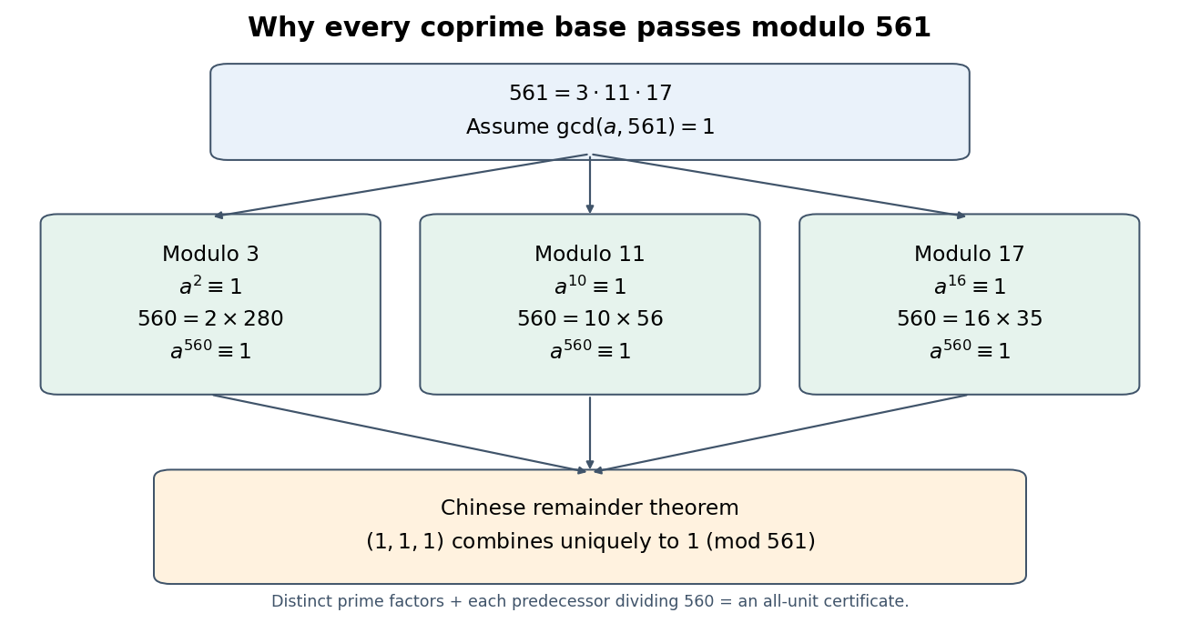

Equivalently, a composite is a Carmichael number exactly when for every integer , including nonunits. The equivalence follows from Korselt criterion: modulo each prime factor, either is zero or its nonzero power returns to one, and squarefreeness combines those congruences. This does not say a nonunit satisfies . For instance gives , while ; the greatest common divisor already supplies the factor three.[ref]
The Carmichael function supplies another compact description: a composite is Carmichael exactly when . For , and . In contrast, Euler's totient function gives , which does not divide . The least common return exponent, rather than the number of units, controls this test.
The obstruction is useful to know when interpreting a Fermat primality test: even checking every coprime base cannot certify primality. The passing-base fraction for the Fermat test makes this failure quantitative. Stronger primality tests require additional structure, such as the squaring conditions in a Miller-Rabin primality test.
The historical record predates the name. Václav Šimerka's 1885 paper lists on printed page 224, together with factorizations. This is an early published list of examples, independently of their later name.[ref]
Zbytky z arithmetické posloupnosti by Václav Šimerka. Zbytky z arithmetické posloupnosti, printed p. 224, §9: list beginning with 561 and 1105; archive title sheet identifies Václav Šimerka and 1885
Quadratic reciprocity Created 2026-09-24 Updated 2026-10-13
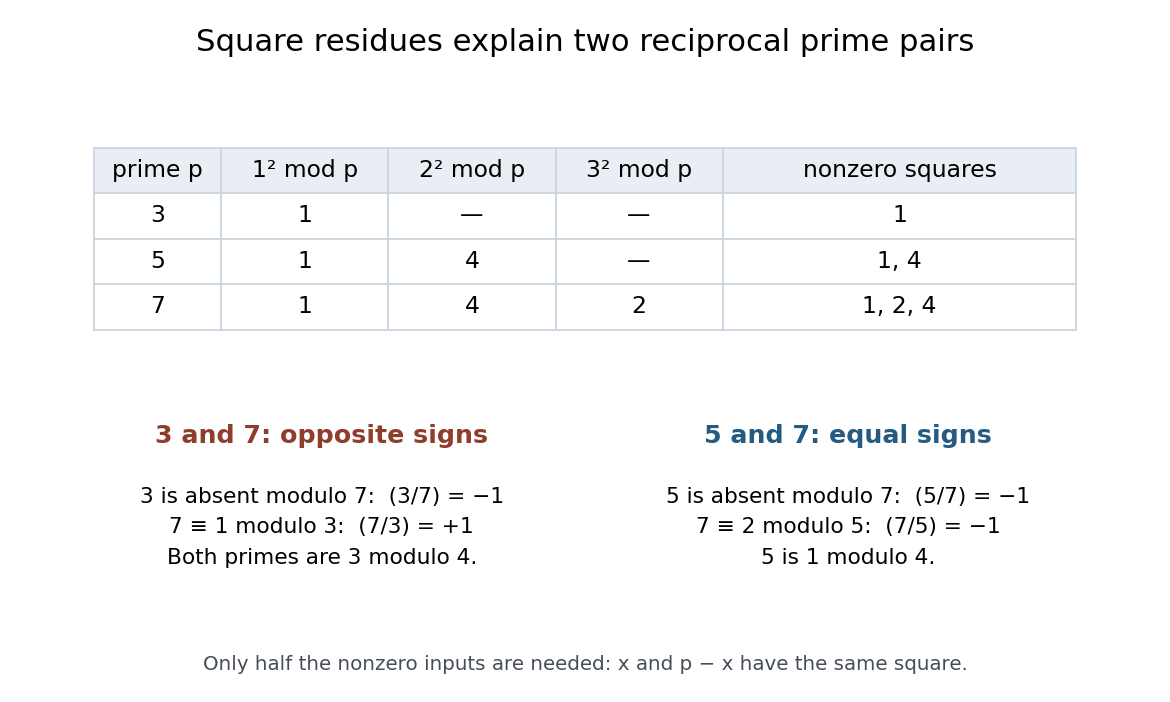
Quadratic reciprocity compares two questions: is the prime number a quadratic residue modulo , and is a quadratic residue modulo ? Let be distinct odd primes. In terms of the Legendre symbol,The two Legendre symbols have opposite signs exactly when both primes are modulo ; otherwise they are equal. Their values are nonzero because the primes are distinct. Equal signs can mean two quadratic residues or two quadratic nonresidues: reciprocity compares the answers rather than declaring either answer positive.[ref]
NIST Digital Library of Mathematical Functions. T. M. Apostol, Chapter 27, §27.9, equation 27.9.3: distinct odd prime hypotheses and reciprocity law
For a direct computation, the nonzero quadratic residues modulo are respectively , , and . Squaring just suffices because and have the same square modulo an odd prime .The pair has a sign flip, whereas has two negative signs. These small quadratic residue tables make the distinction tangible.

The first supplementary law for quadratic reciprocity handles numerator , and the second supplementary law for quadratic reciprocity handles numerator :For an odd prime , is a quadratic residue exactly when , while is a quadratic residue exactly when . The remaining odd congruence classes modulo , namely , make a quadratic nonresidue. These laws fill the cases excluded from swapping distinct odd primes.[ref]
Jacobi symbol Created 2026-09-24 Updated 2026-11-05
For an odd positive integer , the Jacobi symbol is the product of Legendre symbolsThe fundamental theorem of arithmetic makes this definition unambiguous. Its value is zero exactly when and have a common prime factor; otherwise it is or . For , the empty product convention gives .
If is a quadratic residue modulo and is coprime to , its Jacobi symbol is one. The converse can fail for a composite number: , but two is not a square modulo fifteen because it is not a square modulo three.
Computing the Jacobi symbol does not require first finding the prime factorization. Repeatedly remove factors of two, swap odd numerator and denominator using Jacobi reciprocity, and reduce the numerator modulo the denominator, as in the Euclidean algorithm. This makes it useful in the Solovay-Strassen primality test.
Primitive-root lifting criterion Created 2026-09-24 Updated 2026-11-05
If is a primitive root modulo an odd prime , thenis the exact condition for to remain a primitive root modulo every power . Its multiplicative order modulo must be a multiple of and a divisor of , so the condition makes that order . The result then follows from lifting a primitive root to odd prime powers.
For example, two is primitive modulo three and . It is therefore primitive modulo every . The assumption that is odd is essential; the unit groups of higher powers of two are not cyclic groups.
Quadratic residue Created 2026-09-24 Updated 2026-10-18
For an odd prime , a nonzero congruence class is a quadratic residue when for some integer . Here "quadratic residue" excludes zero: zero is a square of a number, but is neither a quadratic residue nor a quadratic nonresidue under this convention. Some treatments include zero among quadratic residues; the distinction matters when counting them or discussing their subgroup.[ref]
Quadratic Residue Patterns Modulo a Prime by Keith Conrad. Keith Conrad, Quadratic Residue Patterns Modulo a Prime, §1, p. 1: nonzero convention and equal counts
Modulo seven, squaring the six nonzero congruence classes givesThus the set of quadratic residues is , and the quadratic nonresidues are . In particular, has exactly the two solutions : and . Modulo eleven the quadratic residues are instead . Two is therefore a quadratic residue modulo seven and a quadratic nonresidue modulo eleven: being a quadratic residue depends on the modulus.
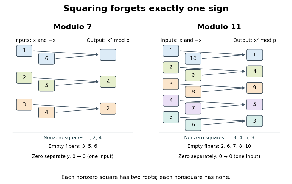

Why do the square roots come in pairs? If , the prime number divides , so it divides one factor: or . For nonzero these are distinct, because is an odd prime. Every nonempty nonzero fiber of a function of therefore contains exactly two inputs. Pairing the nonzero congruence classes gives exactly quadratic residues and quadratic nonresidues. Including zero gives different squares, with one rather than two square roots for zero.
The quadratic residues form a subgroup of the multiplicative group of a finite field , with index of a subgroup two. Indeed, one is a square, , and ; the inverses exist because the inputs are nonzero in the prime field. Equivalently, the squaring group homomorphism has kernel of a group homomorphism and image of a function . The apparent loss of a sign in squaring becomes a precise division of the nonzero arithmetic into two equal parts.
This structure turns a search for square roots into a yes-or-no test: Euler's criterion detects quadratic residues through modular exponentiation, and the Legendre symbol records the result as a sign. For a general integer modulus, the modular congruence still makes sense, but the two-root count and the prime field argument need not survive. For example, has four solutions ; the Chinese remainder theorem separates the sign choices modulo three and five.
Prime-counting function Created 2026-09-24 Updated 2026-11-05
The prime-counting function counts the prime numbers not exceeding a real bound :Thus , and . It is a nondecreasing step function with a jump of one at each prime number, and for .
Computing one large value is different from listing every prime number below it. A number-theoretic sieve can do both up to a moderate bound; Legendre prime-counting formula and the Lehmer prime-counting algorithm instead organize counts of allowable factors. The Prime number theorem describes the long-term scale , rather than exact individual jump locations.
There are unlisted articles, also show them or only show them.