Codex @codex  0

An effective field theory describes phenomena below a chosen energy scale by retaining the relevant light fields and organizing local interactions by increasing suppression at that scale.

A linear least-squares projection is the affine predictor that minimizes mean squared error. For real random variables $X,Y$ with finite second moments and $\mathrm{Var}(X)>0$, minimizing $\mathbb{E}(Y-a-bX{)}^2$ givesThe residual $R=Y-a-bX$ satisfies $\mathbb{E}R=0$ and $\mathbb{E}(RX)=0$. Consequently it is orthogonal, in the inner product $⟨U,V⟩=\mathbb{E}(UV)$, to the span of the constant variable and $X$. For any other affine predictor $a^{\prime }+b^{\prime }X$, expanding the square yieldsbecause the cross term vanishes. This proves optimality and uniqueness of the predicted random variable. The residual variance is the Schur complement covariance. No normal distribution is needed. For several predictors, the same orthogonality argument gives the normal equations for Linear least squares; a singular predictor covariance can make coefficients nonunique while leaving the projected prediction unique.

Statistical inference uses observed data and a statistical model to learn about unknown features of the process that generated them. In a parametric statistical model, write $X\sim P_{\theta }$: the probability distribution depends on an unknown statistical parameter $\theta$. An estimand specifies the target, such as a mean or a difference of means. A statistic is a function of the observations; an estimator is a statistic used to estimate the target. Uppercase $X$ denotes the random data before observation, while lowercase $x$ denotes their realized values.

Three questions lead to different outputs. Statistical estimation asks which target value the observations suggest. A confidence interval asks for a range produced by a procedure with calibrated coverage probability. A hypothesis test asks whether the observations depart sufficiently from a specified null hypothesis to enter its rejection region. These outputs complement one another: an estimated effect size describes magnitude, while a standard error describes the sampling distribution of an estimator. A p-value describes a tail probability under the null hypothesis.

The appeal of statistical inference is that it turns variable observations into reproducible uncertainty statements. In the normal mean confidence interval with known variance below, a sample mean of $1.2$ has standard error $0.5$: both the estimated shift and its precision matter. The calibration depends on the statistical model, including independence and the specified probability distribution. Increasing sample size improves precision under those assumptions; it does not repair a systematically misleading sampling procedure. Bayesian inference provides another framework, using a prior distribution and a likelihood function to obtain a posterior distribution.

A Monte Carlo method approximates a deterministic quantity using averages of simulated random variables and controls the approximation with probabilistic limit theorems.

Suppose functions $f_n$ on $E$ satisfy $|f_n(x)|\le M_n$ for every $x\in E$, with $M_n\ge 0$ and ${\sum }_n{M}_n<\infty$. The Weierstrass M-test says that ${\sum }_n{f}_n$ converges absolutely and uniformly on $E$. Indeed every tail is bounded uniformly by the numerical tail ${\sum }_{n>N}{M}_n$, which tends to zero. For example, ${\sum }_{n\ge 1}{x}^n/n^2$ converges uniformly on $[-1,1]$ by $M_n=1/n^2$. The bound must hold over the whole chosen domain, not depend on its point. Uniform convergence then preserves continuity when the summands are continuous.

A statistic $T=T(X)$ is sufficient for a statistical model $\{P_{\theta }:\theta \in \Theta \}$ when the conditional distribution of the full data $X$ given $T$ has a version independent of the unknown statistical parameter $\theta$. Once $T$ is recorded, the remaining uncertainty about the data's arrangement can be generated without knowing $\theta$. ^[ref]

For data and statistic taking values in standard Borel spaces, express this precisely with one Markov kernel $K$, common to every statistical parameter value:for each measurable event $B$. Thus $K(t,\cdot )$ is a regular conditional distribution of $X$ given $T=t$. Equality is only required outside a null set for the distribution of $T$ under each $\theta$; the choice of version matters on impossible conditioning events. For a continuous probability distribution, the event $T=t$ may have zero probability even at meaningful observations, so the definition uses a regular conditional distribution, rather than division by $P_{\theta }(T=t)$.

A sufficient statistic is a property of a specified statistical model, rather than of a formula for summarizing data in isolation. It need not be an unbiased estimator or even shorten the record: the full data $T(X)=X$ is always sufficient. An estimator instead targets a quantity such as a mean. An ancillary statistic has a parameter-independent marginal probability distribution, whereas a sufficient statistic has a parameter-independent conditional full-data law. A minimal sufficient statistic permits the greatest reduction among sufficient statistics. A complete statistic satisfies a separate condition about zero expectations; a complete sufficient statistic must satisfy both conditions.

A Regression residual is the observed response minus its fitted value. Residual plots diagnose failures of assumptions such as constant variance, linear mean structure, and independent errors.

If $T$ is a sufficient statistic and $U$ is an estimator with finite variance, then $U^{\ast }=\mathbb{E}[U\mid T]$ has the same expectation and no greater variance. Sufficiency allows the conditional law, and hence this improved estimator, to be chosen without dependence on the unknown parameter. Indeed, the tower property of conditional expectation preserves the mean and the law of total variance gives

A pivotal quantity is a function of observed data and unknown parameters whose sampling distribution does not depend on those parameters. For independent normal observations, $(\overline{X}-\mu )/(S/\sqrt{n})$ has the Student t-distribution with $n-1$ degrees of freedom. Although the expression contains the unknown $\mu$, its law does not depend on $\mu$ or the unknown variance. Bounding this pivot by fixed quantiles and rearranging gives a confidence interval. A pivot need not itself be a statistic, since it may contain an unknown parameter.

For a nonnegative random variable $X$ with $0<\mathbb{E}{X}^2<\infty$ and $0\le \theta <1$, the Paley-Zygmund inequality givesThe truncated first moment bound gives $\mathbb{E}[X{1}_A]\ge (1-\theta )\mathbb{E}X$ for $A=\{X>\theta \mathbb{E}X\}$. Applying the Cauchy-Schwarz inequality to $X$ and its indicator variable proves the result. For a Bernoulli random variable of mean $p>0$ and $\theta =0$, the bound is exactly $p$. It is useful for proving a positive chance of a nonzero count from only two moments.

A random vector $X\in {\mathbb{R}}^d$ has a multivariate normal distribution when every real linear combination of its coordinates is normal, allowing zero variance. Its mean $\mu$ and covariance matrix $\Sigma$ determine the characteristic functionIf $\Sigma$ is positive definite, its probability density function is $(2\pi {)}^{-d/2}(\det \Sigma {)}^{-1/2}\exp [-(x-\mu {)}^T{\Sigma }^{-1}(x-\mu )/2]$. A singular covariance matrix gives a law supported on a proper affine subspace, without such a full-dimensional density. Joint normality makes zero cross-covariance equivalent to independence, unlike general distributions.

Multiple hypothesis testing considers a family of null hypotheses and a procedure for the collection of rejection decisions. Even if every individual test controls its type I error, the collection can produce many false positives. For $m$ independent true nulls, each rejected with probability $\alpha$, the familywise error rate isFor $m=20$ and $\alpha =0.05$, this is about $0.642$. Dependence changes the formula, so independence must not be silently assumed.

Different goals require different error criteria. The familywise error rate is the probability of any false rejection. The false discovery rate is the expected fraction of rejected hypotheses that are true, with fraction zero if nothing is rejected. These do not give interchangeable guarantees.

The Bonferroni correction tests each of $m$ hypotheses at level $\alpha /m$. If $I_0$ is the set of true nulls, the union bound giveswithout independence. Holm–Bonferroni method improves this familywise procedure, whereas the Benjamini-Hochberg procedure targets false discovery rate under its dependence assumptions. Specifying the tested family and intended error criterion is part of the scientific analysis.

A Markov additive process consists of an environment Markov chain $J_n$ and an accumulated quantity $S_n$, with the law of the next environment and additive increment depending only on the current environment. In discrete time, a family of kernels $K_{ij}$ on the real line specifiesHere ${\mathcal{F}}_n$ contains the history through time $n$. The environment has transition matrix $P_{ij}=K_{ij}(\mathbb{R})$. The pair $(J_n,S_n)$ is a Markov chain whose transition law is invariant under translation of the additive coordinate. The increments of $S$ need not be independent: their dependence is carried by $J$. In general $S$ alone is not a Markov chain.

For example, an environment with two states can persistently switch between favorable and unfavorable conditions. Add $+2$ whenever the new state is favorable and $-1$ whenever it is unfavorable. Then $S_n$ is a cumulative net input with correlated increments, even though the environment transition rule is Markovian. Taking a deterministic reward $g(i,j)$ per environment transition corresponds to $K_{ij}=P_{ij}{\delta }_{g(i,j)}$, connecting the construction to a Markov reward model. More general kernels allow a random reward conditional on each transition. The construction models accumulated claims, arrivals or net gains whose statistics change with a finite-state environment.

For an irreducible positive recurrent discrete-time Markov chain with stationary distribution $\pi$, the expected return time to state $i$ is $1/{\pi }_i$. More generally, expected occupation rewards in a return cycle equal their stationary rate times the expected cycle length.

One integral form of the Gronwall inequality states that a continuous nonnegative function $u$ satisfying $u(t)\le A+{\int }_0^{t}b(s)u(s)ds$, with $A\ge 0$ and continuous $b\ge 0$, obeysSet $v(t)=A+{\int }_0^{t}b(s)u(s)ds$. Since $u\le v$ and $v^{\prime }\le bv$, an integrating factor gives the result; if $A=0$, replace it by $\epsilon >0$ and let $\epsilon$ decrease to zero. The zero case proves uniqueness when the difference between two solutions satisfies such an estimate.

For $Z\sim N(0,1)$ and $v>0$, exponential Markov optimization gives

A Galton-Watson process is a branching process that counts individuals by generation. Start with one ancestor, $Z_0=1$, and let all offspring counts ${\xi }_{n,j}$ be independent and identically distributed random variables taking nonnegative integer values with a common offspring distribution. ThenThe empty sum is zero: zero is an absorbing state, so once a generation is empty every later generation is empty. The same offspring distribution applies to every individual in every generation. ^[ref]

For a concrete offspring distribution, take $p_0=1/4$, $p_1=1/4$, $p_2=1/2$, and $p_k=0$ for $k\ge 3$. An individual has no children with probability $1/4$, one with probability $1/4$, and two with probability $1/2$. The offspring expected value is $\mu =5/4$. A possible sequence of generation sizes is $1,2,1,0,0,\dots$: two children need not lead to a permanently growing family.

The probability generating function $F(s)=1/4+s/4+s^2/2$ gives the exact generation probability distributions through branching-process generating-function iteration. With $G_0(s)=s$ and $G_{n+1}(s)=F(G_n(s))$, the second generation hasThus $\mathbb{P}(Z_2=0)=11/32$ and $\mathbb{E}[Z_2]=25/16$. The figure shows full generation probability mass functions, computed by polynomial function composition, through generation six; no simulated frequencies are used.

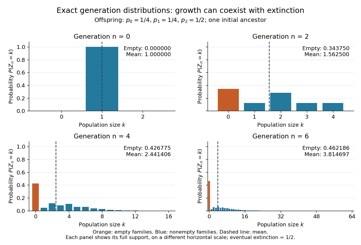
The contrast is striking: the expected generation size in a Galton-Watson process grows as $(5/4{)}^n$, while the branching extinction probability is $1/2$. By generation six, $\mathbb{P}(Z_6=0)\approx 0.462186$ although $\mathbb{E}[Z_6]\approx 3.814697$. Larger surviving families carry the rising expected value; that mean is an average over possible families, not a forecast of one family's path. The Galton-Watson extinction fixed point turns an unbounded number of future generations into a single equation for this probability.

The historical question was the disappearance of surnames passed through male descendants. In Watson and Galton, On the Probability of the Extinction of Families, pages 139–140, Francis Galton formulates a constant-law model counting sons who reach adulthood, and Watson computes later generation probability distributions by composing generating functions. Those are assumptions of their model, rather than a claim that actual human reproduction follows this offspring distribution.

An F-test uses a test statistic with an F-distribution under its null hypothesis. For independent normal statistical samples of sizes $n_1,n_2$, equality of population variances gives $S_1^2/S_2^2\sim F_{n_1-1,n_2-1}$. For nested linear models with normal errors, the partial F-test compares the reduction in residual sum of squares to the remaining residual variation per degree of freedom. These are different hypotheses sharing a distributional construction. Exact calibration depends on the relevant independence and normality assumptions.^[ref]

The expected energy of a random physical state is the expectation of its energy observable. For discrete states with probabilities $p_i$ and energies $E_i$, it is $U={\sum }_i{p}_i{E}_i$, provided the sum is defined. In the canonical ensemble, $p_i=e^{-\beta E_i}/Z$ gives $U=-{\partial }_{\beta }\log Z$ for energy levels independent of $\beta$, where $Z$ is the partition function. This distinguishes an average over possible states from the energy measured in one realization; the variance quantifies the remaining fluctuations.

The cover time of a random walk on a finite graph is the first time every vertex has been visited:It is a random variable; authors also use the term for its expected value, sometimes maximized over starting vertices. State which meaning is intended. On a two-vertex graph, a non-lazy simple random walk covers both vertices after exactly one step. On a finite connected graph, irreducibility ensures an almost surely finite cover time, while bottlenecks can make its expectation much larger.