
Elliptic coordinates Created 2026-09-24 Updated 2026-11-05
Planar elliptic coordinates with focal half-distance are , , with and . Constant positive gives ellipses with foci ; constant gives confocal hyperbolas. Differentiation gives orthogonal coordinate directions with common scale factor . Away from coordinate singularities, the planar Laplacian is , useful for separation of variables on elliptic domains.
Distance from a point to a plane Created 2026-09-24 Updated 2026-10-18
The distance from a point to a plane is the shortest Euclidean distance from the given point to any point on the plane. For with nonzero normal vector , a point hasThe numerator is the residual of the plane equation, not yet a length: its size depends on the chosen normal vector. Dividing by that vector's Euclidean norm removes this arbitrary scale.
For the original example and , the normal vector is and . The residual is , so the distance is . Using the equivalent plane equation instead gives numerator and Euclidean norm , hence the same . A point already on the plane has zero residual and zero distance.
Why is the perpendicular route shortest? Let be the closest point on a plane and any other point on it. The displacement is orthogonal to , so the Pythagorean theorem givesEquality holds only for . This is the closest-point principle of orthogonal decomposition, applied after a translation of an affine plane to its direction linear subspace.[ref]
Orthogonal Projection. Interactive Linear Algebra, §6.3.1: Orthogonal decomposition theorem, Closest vector and distance
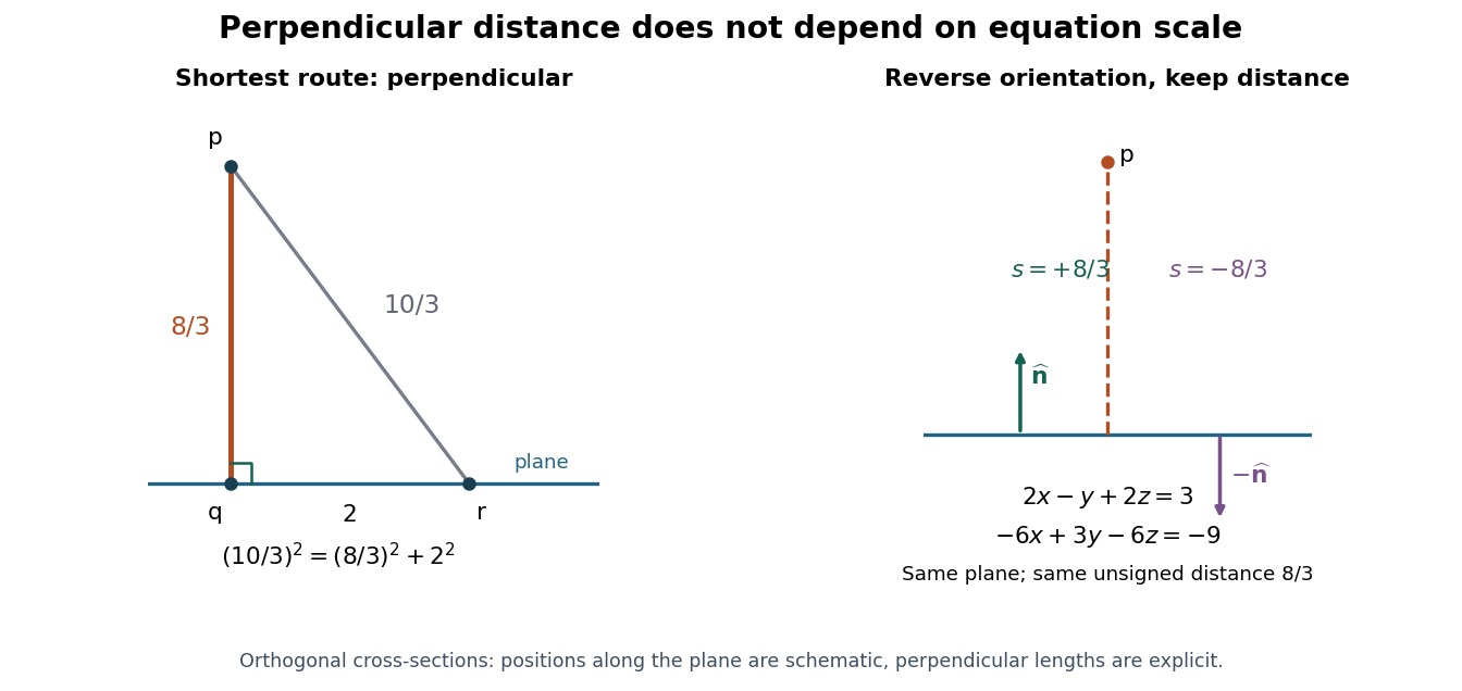
The perpendicular route to a plane is shortest, and rescaling its plane equation preserves the distance
. Original cross-section using the worked distance . The comparison point lies two length units along the plane from the closest point on a plane, giving a longer route of . The second panel reverses the unit normal without moving the plane. Details.
The formula is useful whenever the deviation from a flat reference should be measured geometrically. A raw linear equation residual cannot be compared across arbitrary equation scalings; a perpendicular distance can. The same reasoning works for a hyperplane in any finite-dimensional Euclidean space, with the appropriate number of coordinates.
Connected space Created 2026-09-24 Updated 2026-10-13
A topological space is connected when it has no separation of a topological space: no partition of a set into two nonempty open subsets satisfyingHere the union covers all of , and the intersection is the empty set, so no point belongs to both pieces. For a subset of a larger topological space, "open" means open in the subspace topology: each piece is the intersection of with an ambient open set. Both pieces must be open; merely dividing a drawing into two colours does not establish a separation of a topological space. [ref]
https://math.mit.edu/~hrm/palestine/munkres-topology.pdf. Munkres, Topology: A First Course, section 3-1, definition on p. 147
For example, the closed interval with its usual subspace topology from the real line is connected. The proposed split fails: the second subset is not open in , since every neighbourhood of in contains points less than . More generally, a connected subset of the real line is precisely a real interval. In contrast, for the unionthe open intervals and exhibit as nonempty open subsets in the subspace topology of . Their intersection is empty and their union is , so is not connected. Although are closed intervals in the real line, they are also open within .
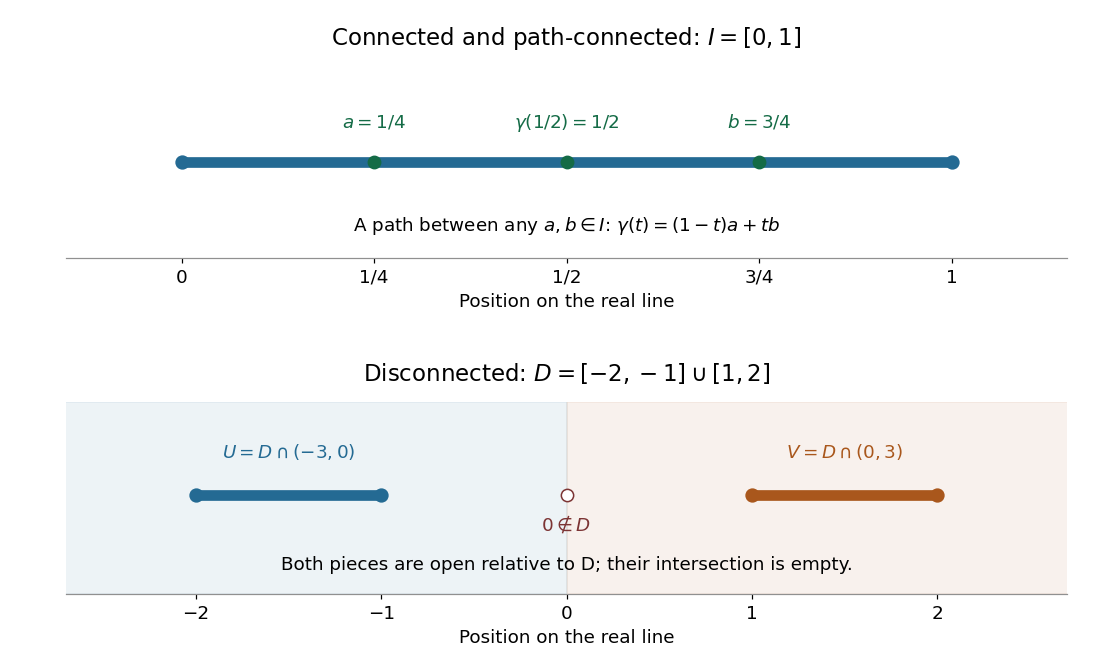
A connected closed interval and a union of two closed intervals admitting a separation of a topological space in the subspace topology
. Details. 
Why is connectedness useful? A continuous image of a connected space is connected: a proposed separation of a topological space in the image would pull back through the continuous map to a forbidden separation of a topological space in its source. Thus a continuous map from a real interval to the real line cannot skip values between two attained values. This is the intermediate value theorem. For a computed example, the continuous function on has image ; the value occurs at . Connectedness guarantees an input attaining that value even when we have no formula for it.
Path connectedness is a stronger condition: it supplies a continuous path between every pair of points. The topologist's sine curve below shows that a connected space need not be a path-connected space.
Conformal map Created 2026-09-24 Updated 2026-11-05
A conformal map preserves angles locally. For differentiable maps between Riemannian manifolds of equal dimension, the condition is with : its derivative scales all directions equally at each point. A holomorphic function in one complex dimension is conformal wherever its derivative is nonzero. For example, is conformal away from zero, but is not globally injective on the punctured complex plane. Local preservation of angles does not require a constant scale or global injectivity.
Classification theorem for surfaces Created 2026-09-24 Updated 2026-11-05
Every closed surface that is connected is homeomorphic to exactly one of a sphere, a connected sum of tori, or a connected sum of real projective planes. The first two cases are orientable; the last is not. Their Euler characteristics are respectively , , and . Thus orientability and Euler characteristic determine the homeomorphism type among closed surfaces that are connected. Compact connected surfaces with boundary are obtained by deleting finitely many disjoint open disks, and the number of boundary components is an additional invariant. This is a classification of spaces, rather than of particular embeddings in three dimensions.
Differential geometry Created 2026-09-24 Updated 2026-10-13
Differential geometry uses calculus to study smooth curves, smooth surfaces, and smooth manifolds. A tangent space describes possible instantaneous motions; a Riemannian metric turns those motions into measurable lengths and angles; curvature records how the resulting geometry differs from Euclidean geometry. Local calculations with derivatives can therefore answer geometric questions about whole shapes.
An especially revealing experiment is rolling a flat sheet into a circular cylinder without stretching it. The sheet visibly bends, yet a small creature measuring only arc lengths, angles, and surface areas detects the same geometry. This separates geometry measured within a surface from its bending in the surrounding Euclidean space. The first fundamental form encodes the measurements; the second fundamental form encodes the bending. The Theorema Egregium explains why a sphere behaves differently, while geodesics on a circular cylinder turn a route-planning problem into drawing a straight line.
Complex geometry Created 2026-09-24 Updated 2026-11-05
Complex geometry studies spaces locally described by complex coordinates with holomorphic transition maps. A complex -dimensional complex manifold has real dimension , but its structure is more restrictive than a smooth atlas: the transition maps satisfy the Cauchy-Riemann equations. The complex projective line is a compact example, described by two complex charts related by . Hermitian metrics and Kähler manifolds connect this analytic structure to Riemannian geometry, while complex algebraic varieties connect it to algebraic geometry.
Algebraic geometry Created 2026-09-24 Updated 2026-11-05
Algebraic geometry studies geometric objects defined by polynomial equations and the algebra of functions on them. For example, defines a parabola, while defines the union of two coordinate lines. The coordinate ring records the second example algebraically: the images of and are nonzero but their product is zero, reflecting two components. Modern schemes extend this dictionary beyond ordinary point sets and permit geometric reasoning over general commutative rings. Applications range from elliptic curves in number theory to families of solutions depending on parameters.[ref]
Algebraic topology Created 2026-09-24 Updated 2026-10-18
Algebraic topology translates questions about topological spaces and continuous maps into questions about groups and other structures from algebra. A topological invariant compresses the enormous amount of data in a space into something one can calculate. For example, the fundamental group records which based loops can be continuously deformed into one another. A filled disk has trivial fundamental group, whereas a circle has fundamental group : an integer remembers how many times a loop goes around.
This compression also respects maps. By functoriality of the fundamental group, a continuous map preserving the chosen basepoints induces a group homomorphism; successive maps induce successive group homomorphisms. Thus geometry supplies arithmetic constraints. A proposed homotopy equivalence must induce an isomorphism, so incompatible fundamental groups rule it out before anyone attempts to construct the deformation.
The beauty is that a whole annulus can retain exactly the same homotopy type as its inner circle. Its thickness disappears under a deformation retraction, while the obstruction to shrinking a loop survives. Equal fundamental groups alone do not establish a homeomorphism or a homotopy equivalence between arbitrary topological spaces.
This turns a visual question into a reusable test. Suppose a continuous map sends the inner circle of an annulus once around another circle. Could it extend over a filled disk spanning that boundary? Such an extension would supply a homotopy shrinking the image loop to a point. Its winding number would have to change from one to zero, which homotopy invariance of winding number forbids. Algebra rules out the extension even when no particular formula for it has been proposed.
Bondi-Sachs formalism Created 2026-09-24 Updated 2026-11-05
The Bondi-Sachs formalism uses outgoing null hypersurfaces to describe gravitational radiation. A null coordinate labels wavefronts, areal radius labels cross-sections, and angular coordinates label null generators.
The Einstein field equations split into radial relations and evolution equations for the angular geometry. At future null infinity, changing Bondi shear gives the Bondi news function, linking radiation to loss of Bondi mass in nonlinear general relativity.[ref]
Bondi-Sachs Formalism by Thomas Mädler and Jeffrey Winicour. Sections 2–3: coordinates, hierarchy and asymptotic radiation
Numerical relativity Created 2026-09-24 Updated 2026-11-05
Numerical relativity computes solutions of the Einstein field equations when an analytic solution or a small-perturbation approximation is insufficient. A 3+1 decomposition of spacetime separates initial spatial geometry and matter from their subsequent evolution. Initial data must satisfy the Hamiltonian constraint and momentum constraint, while the lapse function and shift vector specify the coordinate evolution.
The calculation also needs boundary conditions and a numerical evolution formulation. Resolution studies, constraint monitoring and comparison with known solutions test whether the computed result approximates the intended spacetime. Binary black-hole mergers provide an observational application: numerical waveforms connect strongly dynamical geometry with interferometer signals.[ref]
Observation of Gravitational Waves from a Binary Black Hole Merger by B. P. Abbott and others. Waveform comparison with the predicted inspiral, merger and ringdown
Extracting a physical wave requires controlling the frame and propagation model as well as solving grid equations. Arnowitt-Deser-Misner energy Created 2026-09-24 Updated 2026-11-05
The Arnowitt-Deser-Misner energy is the Hamiltonian boundary charge generating an asymptotic time translation in the ADM formalism. For a spatial metric tensor in asymptotically Cartesian coordinates, use geometrized units :Here is the outward Euclidean unit normal vector. Standard differentiable asymptotic flatness gives and ; suitable additional decay and integrability conditions ensure that the limit exists. Together with ADM momentum, this charge forms the asymptotic energy-momentum four-vector.[ref]
For a time-symmetric Schwarzschild spacetime slice in isotropic coordinates, with . Its surface integrand is . Integrating over therefore gives . The corresponding slice of Minkowski spacetime has constant and zero ADM energy. In a moving asymptotic frame, the energy component need not equal the invariant ADM mass.
Stationary spacetime Created 2026-09-24 Updated 2026-09-24
A stationary spacetime admits a Killing vector field that is timelike in the region representing stationary observers, in particular near infinity for an asymptotically flat stationary black hole.
Black hole Created 2026-09-24 Updated 2026-11-05
A black hole is a region from whose events no future-directed causal curve can reach the distant exterior. In an asymptotically flat spacetime with future null infinity , the standard definition isHere denotes the causal past and is the future event horizon. This is a statement about the complete causal geometry, rather than a material surface or a local force threshold.
For a Schwarzschild black hole, ingoing Eddington-Finkelstein coordinates give outgoing radial null geodesics the slope in units . Inside even this outgoing family moves toward smaller areal radius; the other future radial null family does too. A regular horizon can therefore prevent escape without being a curvature singularity.[ref]
Lecture Notes on General Relativity by Sean M. Carroll. Section 7, Eddington-Finkelstein extension and causal meaning of r=2GM
Rotating examples are described by a Kerr black hole. A dynamically forming event horizon need not coincide with a slice's apparent horizon; locating the former requires global escape information.
Frobenius theorem Created 2026-09-24 Updated 2026-11-05
A constant-rank smooth distribution is an integrable distribution exactly when it is involutive. In differential-form language, let be a local basis of its annihilator, so . The equivalent condition isfor suitable local one-forms . More precisely, the ideal generated by the annihilating forms inside the exterior algebra of differential forms is closed under the exterior derivative; this is an exterior differential ideal. It is not a claim that a two-form lies in the one-form annihilator itself.
For local vector fields tangent to , the definition of exterior derivative givesThus the displayed closure condition says exactly that the Lie bracket of vector fields remains tangent to . The theorem turns this local algebraic condition into integral manifolds through every point.
For a nowhere-zero one-form , its kernel is tangent to local hypersurfaces precisely when . In general relativity, applying this to a metric-dual one-form characterizes hypersurface orthogonality and vanishing twist.
Globally hyperbolic spacetime Created 2026-09-24 Updated 2026-10-14
A globally hyperbolic spacetime has no causal pathologies and admits a Cauchy hypersurface intersected exactly once by every inextendible causal curve.
Null geodesic completeness Created 2026-09-24 Updated 2026-10-13
A spacetime is null-geodesically complete when every inextendible affinely parametrized null geodesic has an affine parameter extending without a finite endpoint in both directions.
A complete manifold requires completeness for every geodesic, whereas this condition only tests null ones.
Null hypersurface Created 2026-09-24 Updated 2026-09-24
A null hypersurface has a degenerate induced metric. Its normal covector raises to a null vector tangent to the hypersurface, whose integral curves are its null generators.
Geodesic congruence Created 2026-09-24 Updated 2026-10-13
A geodesic congruence is a family of nonintersecting geodesics filling an open spacetime region. Its derivative tensor describes the relative motion of neighboring geodesics.
Ricci scalar Created 2026-09-24 Updated 2026-10-03
There are unlisted articles, also show them or only show them.