
The angular momentum eigenstates have eigenvalue , where the angular momentum quantum number is . For each , the magnetic quantum number runs in unit steps from to . Here that magnetic quantum number is , so only half-integer are compatible:Integer cannot contain a eigenvalue . Applying the angular momentum lowering operator and using givesThe lowered vector is nonzero, since the adjoint operator identity givesFinally, is a self-adjoint operator, so its eigenstates for distinct eigenvalues are orthogonal. Explicitly,and hence .
Write and . The canonical commutation relations for the creation and annihilation operators giveFor example, . The expression for from part (b), with distinct modes reordered, then yieldsThus is an invariant subspace, and the matrix of in the ordered orthonormal basis isIts characteristic polynomial is , giving the eigenvalues and normalized eigenstatesIndeed, and by the assumed orthonormality. Both eigenstates remain in the eigenspace.
The common Fock vacuum obeys . Put . By the commutator product rule and part (a),Moving through therefore givesDividing by provesThe constructed number state is nonzero: the relation follows from and . Commuting different modes and successively moving each creation operator across the inner product yieldsThus the given factorial denominator also gives unit norm, as expected for a number state.
From part (a), and . The commutator product rule givesConsequentlyEach term in transfers one excitation between the two modes, preserving the total number operator eigenvalue. This is an instance of the oscillator bilinear commutator; every number operator eigenspace is an invariant subspace of .
Inverting the definitions of the creation and annihilation operators givesSubstituting in the orbital angular momentum givesOperators belonging to distinct modes commute. Therefore the terms with two annihilation operators and those with two creation operators cancel, and , . The surviving terms give the orbital angular momentum in oscillator ladder operators:
First apply the commutator product rule in the form :Repeated use of the commutator product rule gives, for ,This is the commutator with powers of an eigenoperator. For , the commutator with the identity operator is zero, agreeing with the formula.
Each is unchanged by taking the adjoint operator, so in this algebra. Taking the adjoint of a commutator yields . By antisymmetry,In particular, each creation operator raises the number operator eigenvalue by one, and each annihilation operator lowers it by one.
The position operators and momentum operators are self-adjoint operators. Using conjugate linearity of the adjoint operator, , givesWrite . Bilinearity and antisymmetry of the commutator, together with the canonical commutation relations, give . HenceThe terms involving two position operators or two momentum operators vanish by the canonical commutation relations. Finally, reversing products under the adjoint operator, , gives . ThereforeHere is the identity operator. These are the relations for two independent pairs of creation and annihilation operators. The operator algebra in this question is understood on a common invariant operator domain, such as finite linear combinations of the number states constructed in part (c).
The parity operator exchanges and . Their coefficients in the wavefunction are equal, soThus the wavefunction is a parity operator eigenstate with eigenvalue at every time. The orthogonal projection onto the eigenspace is , which annihilates it. By the Born rule,
For a position measurement, the Born rule integrates the probability density over the chosen interval. The three terms from part (b) have integralsandThusThe oscillating term comes from quantum interference between the zero and positive energy components. The probability lies between and , both within ; integrating the same probability density over the whole circle gives one.
The coefficient of the momentum eigenstate is . The Born rule therefore gives . Conditional on this outcome, the projective measurement prepares the post-measurement state , equivalent to up to global phase.
Since , the subsequent energy measurement has conditional probability one of giving the specified energy eigenvalue. The probability for the entire sequence is consequentlyAny intervening unitary time evolution under the same Hamiltonian operator preserves this energy eigenstate, up to global phase.
The ground state is the single energy eigenstate . Its coefficient in the normalized wavefunction is , so the Born rule givesThis probability is independent of because unitary time evolution changes only the dynamical phases of the energy eigenstates.
Since , applying the Hamiltonian operator givesThus the energy eigenvalues and corresponding full stationary states areThe ground state is with energy zero and quantum degeneracy one. For each , the positive energy level has quantum degeneracy two: its energy eigenspace is . This is the free particle spectrum on a circle.
For a momentum eigenstate with eigenvalue , the equation has solution . The periodic boundary condition imposes , so . The wavefunction normalization gives . Choosing a convenient global phase yieldsThese momentum eigenstates form an orthonormal basis, the Fourier basis for the particle on a circle:Here is the Kronecker delta.
For a free particle, the Hamiltonian operator is , where is the momentum operator. The time-independent Schrödinger equation is thereforeThe full stationary state is . The periodic boundary condition identifies and , giving a particle on a circle with wavefunction normalization over one period.
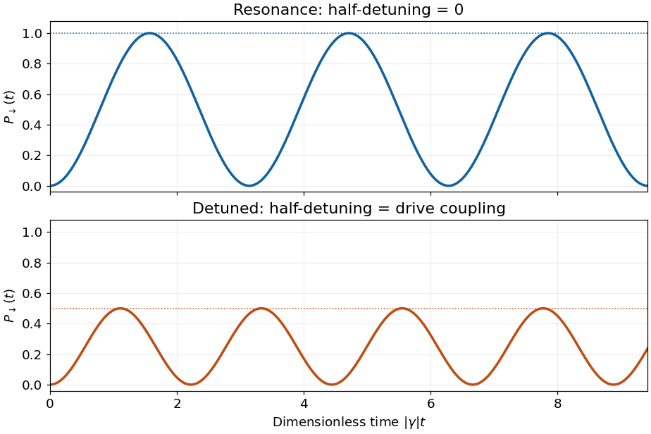
For nonzero Rabi detuning,The sketch starts at zero and oscillates between zero and , with period when the coupling is nonzero. Relative to resonance, the oscillations have a smaller maximum and a shorter period at fixed coupling. The sign of the Rabi detuning changes the amplitudes' phases but leaves this transition probability unchanged. For , its maximum is approximately , so population transfer is strongly suppressed. The plotted detuned example has , giving maximum .
On Rabi resonance, and , soFor nonzero drive the probability starts at zero, reaches unity at , and repeats with period . The population oscillation therefore has angular frequency . This is complete resonant Rabi transfer; a drive of zero strength gives no transition.
Past exam of the quantum field theory course of the University of Oxford 2025 2 c iii Solution 2026-10-25
With the conventional particle labels, the allowed cubic decay channels areEach has one tree-level Feynman diagram, consisting of one cubic Feynman vertex. The final identical-leg contractions supply and cancel the in the Lagrangian density.
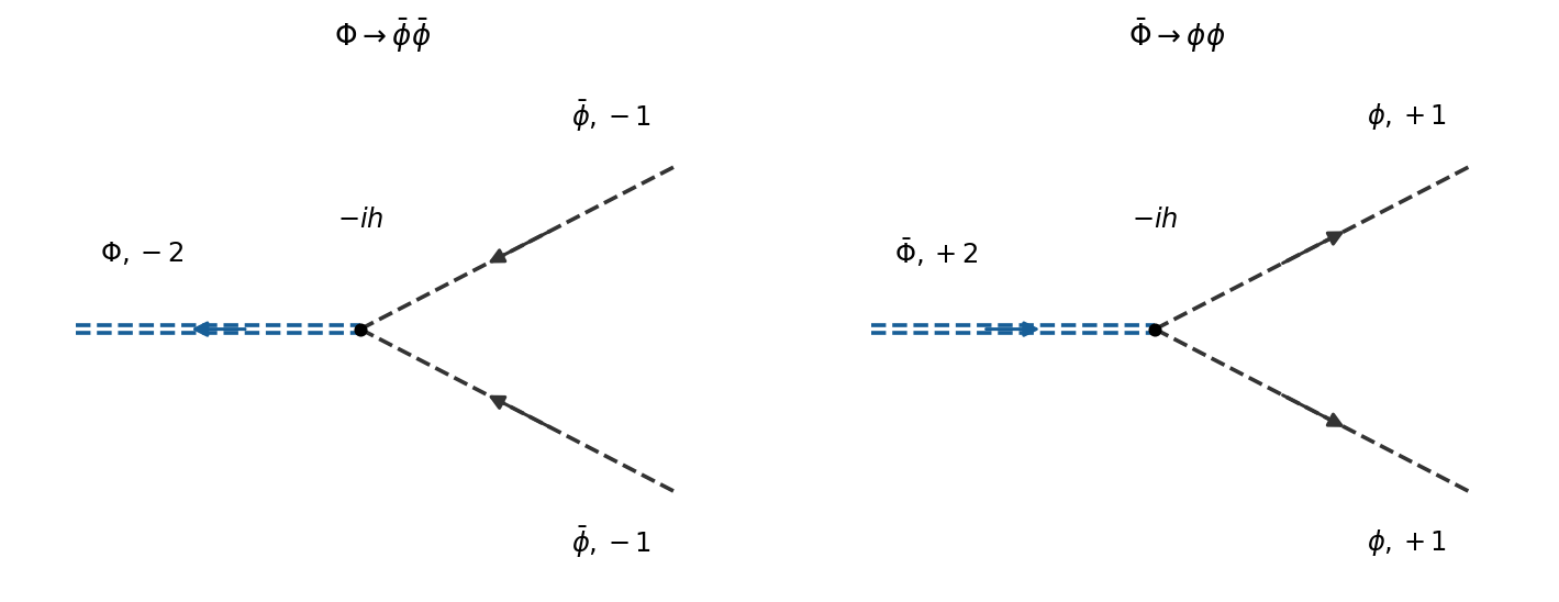
The two charge-conjugate heavy-scalar decays, with explicit antiparticle labels and conserved charge arrows
. Details. Taken literally with these labels, the printed channel is forbidden: its initial Noether charge is and its final Noether charge is . Its decay amplitude is zero, at every order preserving the global phase symmetry. If the source uses “” to name the heavy antiparticle instead, its intended answer is the nonzero decay amplitude for . The following decay width calculation concerns either allowed channel, whose widths are equal by charge conjugation.
Past exam of the quantum field theory course of the University of Oxford 2025 2 c ii Solution 2026-10-25
Keep the particle labels specified under 2. There are two connected tree-level Feynman diagrams: the quartic contact interaction vertex and an -channel light antiparticle exchange. The initial Noether charge is , exactly the charge of . At the first cubic Feynman vertex, the incoming and leave the second leg internal; the conjugate Feynman vertex supplies both outgoing particles.
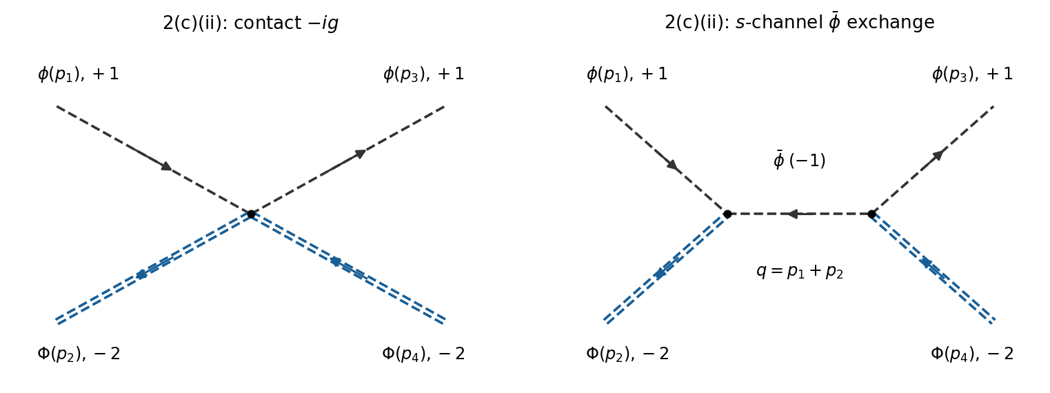
Scattering of a light particle and a heavy particle, with contact and s-channel light-antiparticle exchange diagrams
. Details. The distinction from antiparticles matters. If the paper's heavy “ particle” is instead intended to mean the charge- state , so that its printed decay into is allowed, the exchange diagram is crossed. For that alternative physical process,This is a consistent alternative naming convention only if it is also applied to the decay in iii; one cannot use the same heavy particle label for both charge assignments.
Past exam of the quantum field theory course of the University of Oxford 2025 2 c i Solution 2026-10-25
Let be the incoming and the outgoing four-momenta, and set , , , the Mandelstam variables. The only connected tree-level Feynman diagram is the -channel exchange of , with Noether charge . The two incoming light particles attach to , and the two outgoing light particles to its conjugate. There is no four-light contact Feynman vertex, nor a charge-allowed or exchange with these external labels.
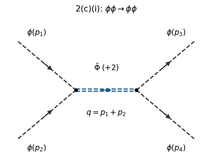


Define the invariant scattering amplitude by . ThenThe Feynman vertices already contain the identical-leg combinatorics. No extra factor of two multiplies this invariant scattering amplitude; the distinct identical final-state symmetry factor enters a cross section integral.
Past exam of the quantum field theory course of the University of Oxford 2023 2 d ii Solution 2026-10-25
Cross the second incoming heavy particle and one outgoing heavy particle in i to obtain . Panel (e) of b's figure shows the resulting box diagram. Its four light-charge arrows again alternate source and sink corners; it is the only connected order- topology. There is no tree exchange because every cubic interaction vertex has only one heavy leg. With , crossing does not affect the zero-external-momentum loop integral, soAn independent check is to integrate out the complex scalar field at constant . Its two real-component squared masses are . The one-loop quantum effective potential is thereforeExpanding the logarithms to fourth order in givesThus the effective Lagrangian has the positive local coefficient . Its external attachments give the common scattering amplitude in both channels. This also checks the box multiplicity and sign.
There are unlisted articles, also show them or only show them.