
Past exam of the fourier analysis course of the University of Oxford 2023 3 a iv Solution 2026-10-25
Use the smooth periodic partition of unity above and define the Fourier coefficients of the periodic distribution byThese are the smooth-window Fourier coefficients of a periodic distribution for period . The finite Schwartz seminorm bound for , restricted to the fixed compact support of , gives for some . Indeed, only finitely many derivatives of occur, and each contributes at most a fixed power of .
For a Schwartz function , the preceding Fourier series formula and yieldAll derivatives of this series converge uniformly. The localization formula in the previous answer therefore givesConsequently the Fourier transform of a periodic distribution isThe polynomial bound on and rapid decay of make every displayed pairing absolutely convergent. In particular there are no derivatives of Dirac delta distributions in this formula.
The inverse Fourier transform of is . Applying continuous Fourier inversion on tempered distributions to the symmetric partial sums givesExplicitly, for every Schwartz function , the pairing of the partial sum with is , which converges absolutely to . The Fourier transform formula also proves that is independent of the chosen smooth periodic partition of unity. For a locally integrable periodic function it reduces, by splitting the integral into periods, to .
Past exam of the fourier analysis course of the University of Oxford 2023 3 a iii Solution 2026-10-25
Let be the Dirac comb. Pair the given identity with the Schwartz function . On the left this gives . On the right,Therefore the Fourier series isThe Fourier bounds for Schwartz functions imply for every . For each nonnegative integer , choose to obtain . Thus the Fourier series and every differentiated Fourier series converge absolutely and uniformly on all of . In particular convergence holds in the topology of smooth periodic functions, defined by uniform convergence of every derivative on one period, and also in tempered distributions.
Past exam of the fourier analysis course of the University of Oxford 2023 3 a ii Solution 2026-10-25
A distribution is a periodic distribution whenIteration gives invariance under all integer multiples of . For a tempered distribution the identity also holds for every Schwartz function, since test functions are dense in the Schwartz space: multiplying by cutoff functions equal to one near zero gives such an approximation in every Schwartz seminorm.
For define . The smooth periodic partition of unity gives with convergence in the Schwartz space. Indeed, each is supported where , and the generalized Leibniz rule and arbitrarily rapid decay of the derivatives of give, for every ,Consequently continuity and periodicity of the tempered distribution giveFor the last interchange, all summands have the fixed compact support of and their derivatives decrease faster than any power of . Hence the series converges in the space of test functions, as well as in the Schwartz space. Notice that itself need not be a Schwartz function; the factor makes the pairing legitimate.
The periodization of a Schwartz function isFor every nonnegative integer , the Schwartz seminorms give uniformly for . The Weierstrass M-test gives absolute and uniform convergence there of the defining series and all its differentiated series. Termwise differentiation proves that is a smooth function, with . Reindexing the absolutely convergent series proves , so it is a periodic function.
For an explicit smooth periodic partition of unity, choose the bump functionIt is a test function, positive on . The smooth function is periodic and strictly positive, since every has a translate in . SetDivision preserves smoothness because , and the support remains contained in .
Past exam of the fourier analysis course of the University of Oxford 2023 2 b iii Solution 2026-10-25
Write , , and . By the Sobolev space hypotheses, and belong to the L2 space. Their product is an integrable function by Cauchy-Schwarz inequality. Thus is a locally integrable function defining a tempered distribution, with estimateThe supremum is controlled by finitely many Schwartz seminorms. Define the convolution of Sobolev distributions byIt is independent of the representatives chosen for , and the convolution theorem shows that it agrees with ordinary convolution for Schwartz functions. More generally, approximate by Schwartz functions in their respective Sobolev norms; the displayed estimate shows convergence of the products in tempered distributions, so their ordinary convolutions converge to this definition. For that also satisfy the stated Sobolev space hypotheses, the ordinary convolution theorem gives the same result.
There need not be any real with . ChooseHere is an indicator function. Since and every weight is bounded above and below by positive constants on , both and belong to every Sobolev space. But their convolution has Fourier transform , and for every real ,Thus . The obstruction is failure of local square integrability at zero; a weight controlling large frequencies cannot fix it.
Past exam of the fourier analysis course of the University of Oxford 2023 2 b ii Solution 2026-10-25
The distributional derivative is defined by . Since differentiation under the integral sign gives , we obtainThis proves the Fourier transform of a derivative identity for all tempered distributions.
If , their Fourier transforms are represented by locally square-integrable functions, and the identity identifies with almost everywhere. Hence the Sobolev norms satisfyso for every real .
For real , the Sobolev space consists of those tempered distributions whose Fourier transform is represented by a locally square-integrable function and for whichThis is the Sobolev norm used here; inserting the fixed factor gives an equivalent convention.
For the constant function , Fourier inversion at zero givesA nonzero Dirac delta distribution cannot be represented by a locally square-integrable function. Indeed, if represented , choose a test function with , and put . On a fixed compact interval containing their supports, Cauchy-Schwarz inequality givesThus . Every Sobolev space requires local square integrability of the Fourier transform, regardless of how negative is. ThereforeThe zero constant function belongs to every Sobolev space.
Past exam of the fourier analysis course of the University of Oxford 2023 2 a ii Solution 2026-10-25
Set . This is a Schwartz function and its Fourier transform is . The convolution theorem givesThe convolution of two Schwartz functions is again a Schwartz function: differentiating under the integral and expanding bounds every weighted derivative by products of integrable and bounded weighted derivatives. Evaluate Fourier inversion for this convolution at zero:The Schwartz space is dense in the L2 space. For choose Schwartz functions in the L2 norm. The identity makes a Cauchy sequence in the L2 space, and its limit defines , independently of the approximation. It agrees with the distributional Fourier transform, because Cauchy-Schwarz inequality makes convergence in the L2 norm imply convergence when paired with every Schwartz function. For it therefore agrees almost everywhere with the ordinary Fourier transform.
The extension is onto: its image is closed by the norm identity and contains the Schwartz space, since Fourier inversion maps that space to itself. This proves Plancherel theorem:Its inverse is the extension of the inverse Fourier transform, with limits understood in the L2 norm.
Let , and define reflection of a tempered distribution by . The Fourier inversion theorem on the Schwartz space says . ThusReflection commutes with the Fourier transform, since and the same relation follows by duality for tempered distributions. Define the inverse Fourier transform on tempered distributions byIt follows thatIn particular is the general Fourier inversion formula. When is an integrable function, this is the regular distribution of ; an arbitrary tempered distribution need not have an ordinary integral representation.
Past exam of the fourier analysis course of the University of Oxford 2023 1 b ii Solution 2026-10-25
If , then is an integrable function, so the Riemann-Lebesgue lemma supplies a continuous representative of its Fourier transform. Equivalently, in the mixture for the majorant is integrable at zero precisely when . In this case dominated convergence also givesIf , Fatou's lemma applied along any sequence of nonzero tending to zero givesThe divergence comes from zero, where the exponent is at most . A continuous representative would agree with almost everywhere. Since both are continuous on each open half-line, they must agree everywhere on those half-lines: a nonzero continuous difference would be nonzero on an interval of positive Lebesgue measure. The displayed blow-up then contradicts continuity of at zero. Changing a value at one point cannot remove this singularity. Consequently
Put . The defining integral of the gamma function, with , givesThe Fourier transform of a Gaussian suggests the following representative for the Fourier transform of an inverse power of one plus x squared:All factors are positive. Tonelli's theorem evaluates its total integral, allowing an infinite value at the single point zero:Assign any finite value at zero if necessary. This gives an integrable function with .
To verify equality as tempered distributions, take any Schwartz function . Substituting the mixture into is justified byFor each , Fubini's theorem and the Fourier transform of a Gaussian identify the inner pairing with . Interchanging the resulting integrals is valid because their absolute value is bounded by after integrating the positive kernel. ThereforeFinally, on a compact set with , the mixture integrand is bounded by , which is integrable both at zero and at infinity. Dominated convergence proves continuity there. Hence .
Past exam of the fourier analysis course of the University of Oxford 2023 1 a iii Solution 2026-10-25
A tempered distribution is a continuous linear functional . Equivalently, for some integer and constant ,The Fourier transform of a tempered distribution is defined byThe Fourier bounds for Schwartz functions make the right side a continuous linear functional on the Schwartz space, so is again a tempered distribution.
For an integrable function , the regular distribution acts by . The estimate proves it is a tempered distribution. Since , Fubini's theorem givesThus the distributional Fourier transform agrees with the ordinary Fourier transform.
Past exam of the fourier analysis course of the University of Oxford 2023 1 a ii Solution 2026-10-25
For , insert a Gaussian function into the proposed inverse Fourier transform:The Fourier bounds for Schwartz functions show that is an integrable function, so dominated convergence givesOn the other hand, Fubini's theorem applies because . The given Fourier transform of a Gaussian, rescaled by , yieldsThe last integrand is bounded by . Since is continuous, another application of dominated convergence makes this tend to . Equating the limits proves the Fourier inversion theorem:The Gaussian functions above form an approximate identity; no Fourier inversion was used in evaluating their integrals.
Use the Fourier transform convention , with complex-linear distribution pairings throughout. The Riemann-Lebesgue lemma says that, for an integrable function , its Fourier transform is continuous and tends to zero as . It also satisfies . The product rule, or convolution theorem, isHere belongs to by Tonelli's theorem, and Fubini's theorem proves the displayed identity. The companion Fourier product formula, for Schwartz functions, is .
A Schwartz function is a smooth function for which every Schwartz seminormis finite. These seminorms define the topology of the Schwartz space . In particular,Thus every Schwartz function is an integrable function.
The Fourier bounds for Schwartz functions assert that each Schwartz seminorm of is bounded by finitely many Schwartz seminorms of . Explicitly, differentiation under the integral sign and integration by parts giveso the generalized Leibniz rule and the preceding integrability estimate giveIn particular the Fourier transform maps the Schwartz space continuously into itself.
Taking the imaginary part of the complex potential gives the streamfunctionThe corresponding velocity field isPut . Then and . Thus the streamlines are the previous rectangular hyperbolas rotated clockwise by . Their separatrices have angles ; the extension axis is and the compression axis is perpendicular to it. The middle panel of the figure shows this rotation.
For pure advection, a marked fluid element obeysConsequently the dye circle becomes an ellipse with semiaxes and . Its area isStretching in one principal direction exactly compensates compression in the other. Equivalently the flow-map Jacobian determinant is one, as required by incompressibility. Negligible diffusion is needed to regard the sharp dye boundary as a material curve.
Using and the complex velocity convention ,The streamlines are , a family of rectangular hyperbolas whose asymptotes are the coordinate axes. The origin is a stagnation point. Fluid moves inward along the axis and outward along the axis, with the same directions approached by the neighbouring streamlines. This is a planar extensional incompressible flow, illustrated in the left panel below.
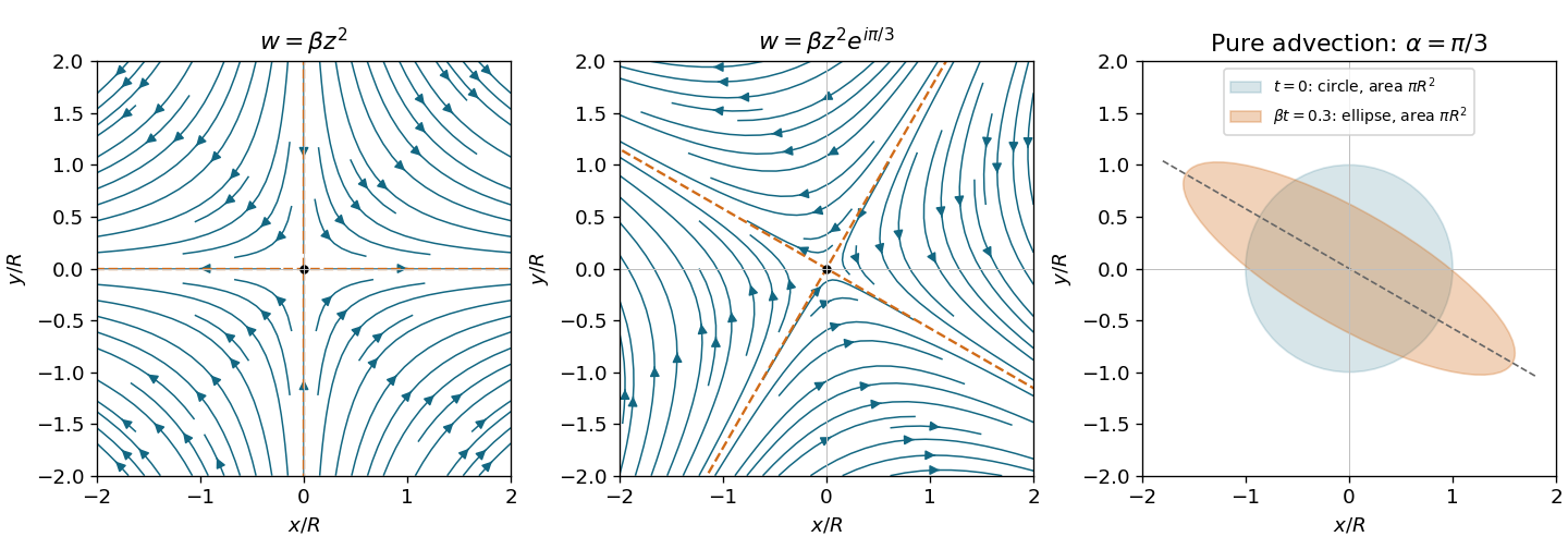
Quadratic complex potentials give hyperbolic streamlines and area-preserving dye deformation
. Original streamlines for zero phase and phase , with arrows from the analytic velocity fields. The principal extension axis rotates by . The right panel compares a unit dye circle with its image at for ; the ellipse has the same area. Details.
Past exam of the fluids and waves course of the University of Oxford 2023 3 c ii Solution 2026-10-25
Define the dimensionless parameterThe stipulated hierarchy implies both andThus the finite-depth correction uses , while the restoring effect of bending stiffness is small compared with gravity. The dispersion relation becomesHence, to leading order, these surface gravity waves are nondispersive waves withFor clarity, the first corrections to the phase speed areThey exhibit the weak residual wave dispersion at finite wavenumber. The claimed nondispersive behavior is the asymptotic leading-order result, not exact equality for the complete relation.
In the deep-water limit , . Put . The squared phase speed of the flexural-gravity wave is thenIt diverges as and as in this limiting model. Its unique stationary point satisfiesThe second derivative is positive. Using gives the minimum phase speed of a flexural-gravity wave:This is the deep-water minimum: applying it to a finite depth requires . Otherwise the factor must be retained in the minimization. Within the deep-water approximation, phase speed and group velocity coincide at , although the wave family remains dispersive.
Past exam of the fluids and waves course of the University of Oxford 2023 3 b iv Solution 2026-10-25
Let , with . The surface elevation is , so . Use separation of variables in the interior Laplace equation:The term is excluded by the bed no-penetration boundary condition. The linear surface kinematic boundary condition determinesAn irrelevant additive constant is omitted. At ,The linear dynamic boundary condition then reduces toConsequently the dispersion relation of a floating elastic plate with zero plate inertia isThe negative-frequency branch gives propagation in the opposite direction. For signed wavenumber, replace by in the squared-frequency formula. Setting recovers the finite-depth surface gravity wave relation, a useful sign check.
Past exam of the fluids and waves course of the University of Oxford 2023 3 b iii Solution 2026-10-25
Linearize about the resting state , . Introduce a dimensionless small parameter and writeholding the depth, bending stiffness and variation scales fixed. Thus both boundary displacement and induced velocity are small. For any first-order derivative , a Taylor expansion at the moving surface givesThe displacement correction to the leading field is , so evaluating it on changes it only at second order. Also and . The first-order kinematic boundary condition and dynamic boundary condition are thereforeDropping the subscript, the linearized boundary condition pair isThe fixed-bed condition remains . The source's shorthand requires a length scale: for the subsequent plane wave, small surface slope and displacement small compared with depth are sufficient conditions. Small height alone, with arbitrarily rapid spatial variation or a finite background disturbance, does not justify discarding the products.
There are unlisted articles, also show them or only show them.