
Use calibrated multispectral imaging of reflected sunlight, with visible, near-infrared and short-wave-infrared bands. A satellite records radiance in several passbands for each ground pixel. Perform geometric registration and atmospheric correction to estimate spectral reflectance, then account for illumination differences on slopes and mask cloud, water and dense vegetation. A false-colour composite, diagnostic band ratios or a trained statistical classification can separate surface lithologies; field observations and representative spectra validate any mapped contact.
Different minerals have different absorption features: iron-bearing materials affect visible/near-infrared spectral reflectance, while hydroxyl-bearing clay minerals and carbonate-bearing rocks can differ in short-wave-infrared bands. Adjacent patches with reproducibly different spectra and coherent geological boundaries are candidates for lithological contacts. This is particularly useful in dry, exposed terrain. Vegetation, soil cover, similar rock compositions, weathering and topographic shadow can hide or mimic a contact; a colour boundary alone is insufficient.
Choose spatial resolution appreciably finer than the narrowest unit being mapped, with several pixels across that unit. Approximately – is suitable for regional contacts separated by hundreds of metres; metre-scale units require finer imagery or field work. Sentinel-2 provides – bands useful for this purpose, while the reflected-light multispectral bands of Landsat are typically . Broad multispectral passbands distinguish many rock assemblages but cannot resolve every narrow mineral absorption feature; hyperspectral imaging is preferable when those features are essential.
Within a shallow fault zone undergoing brittle fracture, repeated sliding crushes and grinds grains. Expect fault gouge, potentially rich in fine clay minerals, and coarser angular fault breccia; a cohesive, cemented crushed rock is a cataclasite. Slickensides or displaced grains can record the sliding direction.
An opening geological joint need not contain any fault rock: it may be an open crack. If fluids circulated, it can contain a mineral vein, for example calcite or quartz, grown from the fracture walls. Thus comminuted fault rock supports shear, while open space or a crack-filling mineral vein supports opening. Mineral filling is conditional on fluid chemistry and timing; its precise composition cannot be inferred from the photograph.
The reverse fault requires strong east–west compression; the vertical opening geological joints require the least principal stress in the effective stress tensor east–west. They need not have formed at the same time or under the same local stress field. Compression can form the reverse fault during burial and crustal shortening; subsequent tectonic exhumation, unloading, relaxation, cooling or another tectonic episode can rotate the principal stress ordering and permit opening geological joints.
Furthermore, local stress near faults, layer interfaces and topography can differ from the regional stress. A high pore pressure shifts every Mohr circle left by , helping tensile failure, but isotropic pore pressure alone cannot exchange the east–west and vertical principal stress ordering. Determine relative timing using cross-cutting relations, offsets of geological joints, and any generations of fracture-filling minerals. Spatial coexistence is therefore evidence of a deformation history, rather than a requirement that the two failure diagrams describe one simultaneous homogeneous stress state.
Use compression-positive effective stress normal to the plane on the horizontal axis and shear stress on the vertical axis. For any chosen pair of principal stresses, Mohr's circle has centre and radius .
For the reverse fault example, and . Draw the two Mohr-Coulomb failure criterion lines . The tangencies areThese are shear failure points with nonzero shear stress. The two smaller three-dimensional Mohr circles use and ; they lie inside the outer circle and do not touch the envelope in this example.
For the opening geological joints, use the tensile failure criterion . The example gives , and . The circle first touches this vertical cutoff at . Thus the geological joints form on planes normal to and have zero resolved shear stress. A complete brittle envelope can combine this tensile cutoff with compressive Mohr-Coulomb failure criterion, using sufficient cohesion that shear failure does not occur first. The failure-mechanics figure displays these two distinct constructions.
Interpret the vertical, apparently unoffset fractures as opening geological joints. Their normals are east–west, so the least principal stress must be east–west and sufficiently tensile in effective stress. The other two principal stresses lie within the vertical north–south geological joint plane; their ordering cannot be recovered from this fracture orientation alone.
One example, with compression positive and coordinates east, north, up, isHere is vertical, north–south, and east–west. The geological joint opens east–west when its tensile strength is . An isotropic pore pressure can make the east–west effective stress tensile even while the total normal stress remains compressive. Draw opening arrows pointing away from the vertical fracture, rather than sliding arrows along it.
The offset layered sequence indicates reverse slip on the west-dipping fault: its western hanging wall moved up relative to the eastern footwall. With the fault strike perpendicular to the east–west image plane, an Andersonian faulting regime has horizontal east–west, horizontal north–south, and vertical. Draw opposing compression arrows east–west and a smaller opposing pair vertically; the intermediate pair points into and out of the page.
For example, in east, north, up coordinates, a compression-positive effective stress tensor consistent with a reverse fault and zero cohesion isThese magnitudes illustrate one possible stress tensor, rather than a measurement from the photograph. With , the – Mohr circle is tangent to the Mohr-Coulomb failure criterion at a plane from horizontal. The original failure-mechanics figure above sketches these principal stress directions.
Extinction debt is future extinction committed by past environmental change but not yet realized because populations persist temporarily. After habitat loss or fragmentation, surviving adults and small isolated populations can remain visible even when successful recruitment and recolonization are too low for long-term persistence. Long generation times can delay the observed species loss.[ref]
Habitat destruction and the extinction debt by David Tilman and others. Abstract: extinctions delayed for generations following habitat fragmentation
Thus current species richness can overstate the diversity sustainable under present habitat conditions. Restoration or renewed connectivity before the delayed losses occur may avert part of the debt; the concept is a lagged consequence of past change, rather than a prediction that every threatened population is irreversibly doomed.
Extinction selectivity means that the probability of extinction depends systematically on biological or ecological traits, rather than being equal across all species. An empirical association needs a specified event, group and taxonomic level; a trait protective in ordinary background turnover may not protect during every mass extinction.
Geographic range: at the end-Cretaceous crisis, geographically widespread marine bivalve genera had lower extinction intensity than narrowly distributed genera. This makes range breadth a demonstrated selective trait for that dataset. The same analysis found no clear selectivity by body size, so that result should not be generalized to every trait or event.[ref]
Selectivity of end-Cretaceous marine bivalve extinctions by David Jablonski and others. Abstract: geographic-range selectivity and absence of body-size selectivity
Body size: large-bodied mammals suffered disproportionately during late-Pleistocene and later Quaternary losses, including the loss of many giant herbivores and carnivores. A global analysis over the last years found strong size-selective losses across continents and trophic modes. Large size can correlate with slow reproduction, high resource demand and exposure to human hunting, but the observed size pattern and its possible mechanisms should be distinguished.[ref]
Body size downgrading of mammals over the late Quaternary by Felisa Smith and others. Abstract: size-selective extinction across continents, trophic modes and intervals
Sexual dimorphism and reproductive investment: a study of fossil cytheroid ostracods found much higher estimated extinction rates in species with stronger male–female carapace dimorphism, interpreted as greater male investment in reproduction. This supplies a third empirical trait association; the observed relationship is not a universal claim that sexual selection is always harmful.[ref]
High male sexual investment as a driver of extinction in fossil ostracods by Maria João Fernandes Martins and others. Abstract and main result: approximately tenfold rate contrast between high- and low-investment species
A mass extinction is driven by changes that overwhelm organisms' physiological tolerances or destroy their food and habitat systems. Distinguish the initiating forcing from the linked environmental mechanisms: one event can generate several contributors.
- Large extraterrestrial impact. At the Cretaceous–Palaeogene boundary, the Chicxulub impact injected dust, aerosols and soot that reduced incoming sunlight and photosynthesis, disrupting food webs; rapid heating, fires and subsequent cooling added stresses. The impact is the trigger, while darkness and loss of primary production are proximate mechanisms.
- Large-scale volcanism. Eruption and intrusion of large igneous provinces, notably the Siberian Traps around the end-Permian crisis, release or mobilize gases and can produce rapid climate change. Carbon dioxide favors warming; sulfur-bearing emissions can cause shorter cooling and acid deposition. The outcome depends on rate, duration and interacting reservoirs, rather than eruption volume alone.
- Ocean anoxia and euxinia. Warming lowers oxygen solubility and can strengthen stratification; altered nutrient supply increases oxygen demand. Oxygen loss removes habitable marine volume, while sulfide in anoxic waters can be toxic. These processes contributed to the end-Permian marine crisis and can reinforce warming-driven mortality.
- Ocean ocean acidification and elevated carbon dioxide. Rapid addition of carbon dioxide changes seawater carbonate chemistry and can impair biomineralization, while high carbon dioxide also challenges physiological acid–base regulation. Susceptibility varies with physiology; this is a linked mechanism rather than proof that every calcifying group responds identically.
- Rapid cooling and eustatic sea level change. Late Ordovician glaciation and regression reduced shallow-marine habitat and changed temperatures and circulation; subsequent warming and oxygen loss introduced a different set of stresses. Habitat loss and climate change can therefore contribute in successive phases of one crisis.
These examples supply more than four drivers or contributors. The historical effects of volcanism, warming, oxygen loss and elevated carbon dioxide can act together rather than compete as mutually exclusive explanations.[ref]
Paleophysiology and end-Permian mass extinction by Andrew H. Knoll and others. Abstract and introduction: linked physiological effects of warming, anoxia, sulfide and hypercapnia
A mass extinction is a geologically brief, geographically widespread loss of a large fraction of species across multiple major groups, substantially exceeding background extinction rates. Severity, global extent and rapidity distinguish it from the disappearance of a local population or the ordinary loss of individual lineages. A threshold near of species is often used operationally, but the qualitative definition does not depend on one universal numerical cutoff. The duration is short on geological timescales, and need not mean that every species disappeared simultaneously in a single day.
Allopatric speciation begins when a geographic barrier divides a population and reduces gene flow. Independent mutation, genetic drift and divergent natural selection can then build reproductive isolation; if populations later meet, they remain distinct when isolation is sufficiently strong. Sister lineages of snapping shrimp in the genus Alpheus on opposite sides of the Isthmus of Panama illustrate the role of separated marine populations. Their divergences are not all synchronous with the final closure: genetic data indicate several separation histories, so one barrier date should not be assigned indiscriminately to every pair.[ref]
New dates and new rates for divergence across the Isthmus of Panama by Nancy Knowlton and others. Abstract: comparisons of 15 trans-isthmian pairs and heterogeneous divergence
Sympatric speciation develops without a geographic barrier separating the initial population. Divergent ecological selection combined with assortative mating, habitat-associated mating, different reproductive times or a chromosomal change can reduce gene flow within a shared area. The palms Howea forsteriana and Howea belmoreana on Lord Howe Island provide a documented candidate: different soil associations and substantially different flowering times contribute to reproductive isolation, and their sister relationship and timing support divergence on the island.[ref]
Sympatric speciation in palms on an oceanic island by Vincent Savolainen and others. Abstract and Figures 2–3: flowering-time and soil associations
The distinction concerns the geography of divergence, not whether present-day ranges overlap. Present coexistence alone cannot distinguish sympatric speciation from earlier allopatric speciation followed by range expansion. Parapatric speciation describes divergence between adjacent populations with limited exchange and provides an intermediate geographical category; the two main modes requested are the allopatric and sympatric endpoints.
The biological species concept groups natural populations that actually or potentially interbreed and are reproductively isolated from other such groups. Its central criterion is reproductive isolation and gene flow, rather than visible similarity. It is hard to apply directly to fossils, organisms reproducing strictly by asexual reproduction, and geographically separated populations whose potential interbreeding cannot be tested.
The phenetic species concept groups organisms by overall similarity in measured phenotypic traits. A practical morphological species concept uses anatomical form as its main evidence; strict phenetic classification can combine many kinds of measured traits. This makes such approaches usable for preserved specimens and much of the fossil record, but the decision depends on which traits are measured and how similarities are weighted.
At least four difficulties arise. Cryptic species may be reproductively isolated while looking nearly identical, so similarity can lump separate lineages. Conversely, sexual dimorphism, juvenile/adult differences and phenotypic plasticity can make one interbreeding species look like several, causing over-splitting. Convergent evolution can make distantly related organisms resemble one another in ecologically selected traits. Finally, continuous geographic or temporal variation supplies no unique gap at which to place a boundary: character choice, sample size, preservation and similarity thresholds can alter the inferred species delimitation. These are distinct from the biological concept's practical difficulty of testing actual interbreeding.
Gregor Mendel's first law is Mendelian segregation: the two alleles at a genetic locus in a diploid individual separate into different gametes, so each gamete receives one. In ordinary meiosis, separation of homologous chromosomes at meiosis I provides the chromosomal mechanism; their sister chromatids separate at meiosis II.
The second law is independent assortment: segregation at one genetic locus is independent of segregation at another when the loci are unlinked. Random orientation of different pairs of homologous chromosomes at meiosis I supplies the mechanism for genes on different chromosomes. Genetic linkage is an essential qualification: nearby loci on one chromosome do not generally assort independently, although sufficiently frequent genetic recombination can make their observed combinations approach independence. Genetic dominance concerns the phenotype of a heterozygote and is not one of these two segregation laws.
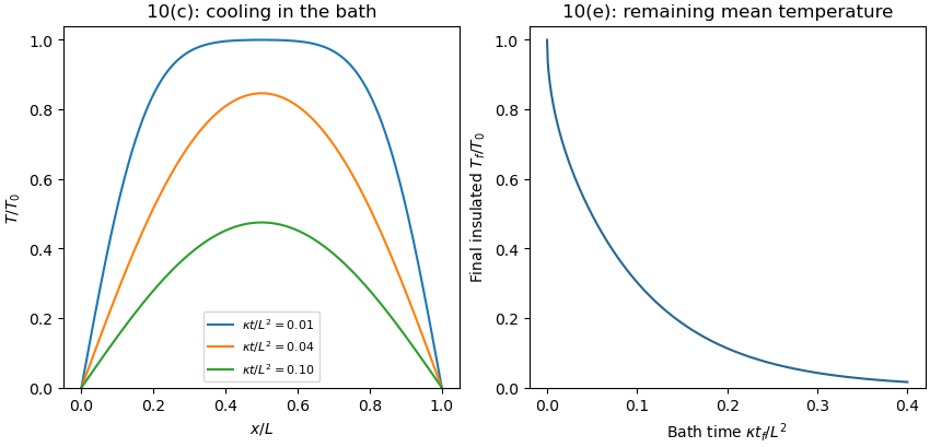
After bath cooling followed by insulated equilibration, the remaining mean temperature is conserved: integrating the insulated heat equation givesFor constant density, specific heat capacity and cross-section, this is conservation of energy. Its Fourier cosine series has a constant mode equal to the initial integral average; every nonconstant mode decays. Therefore the eventual uniform temperature isFor each mode with an odd integer index in part (c), . Integrating the bath-cooled series yieldsFor , uniform convergence justifies termwise integration; the result also follows by dominated convergence of the summable positive coefficients. As a check, gives for zero bath time, and as . More bath time strictly lowers the retained average temperature when and .
Write after removal, with . Neglecting heat loss to air means thermal insulation, rather than an end to internal thermal conduction. The evolution and conditions areHere is the nonuniform bath-cooled profile derived in part (c). At the switching instant it need not have zero endpoint derivatives: the sudden replacement of Dirichlet boundary conditions by Neumann boundary conditions can produce another initial-boundary corner incompatibility. The insulated heat equation nevertheless recovers the given profile and satisfies its new boundary conditions for .
The reference to part “(c)(i)” in the source is circular; the relevant modes are those verified in part (b)(i). Linearity of the heat equation and its homogeneous Dirichlet boundary conditions allows superposition of those modes:Match the initial uniform interior temperature using the orthogonality of the Fourier sine series:Thus for even integers and for odd integers , givingFor every , the exponential factor makes the series and the derivatives needed in the heat equation converge uniformly on later time intervals. At , the Fourier sine series equals at interior points but zero at the endpoints: the instantaneous cooling boundary condition is incompatible with the pre-immersion endpoint values. This corner mismatch is physically the idealization of an instantaneous bath contact and does not invalidate the solution for .

There are unlisted articles, also show them or only show them.