
Cathode-ray oscilloscope Created 2026-10-18 Updated 2026-10-20
Oscilloscope probe 2026-10-18
A connection that couples a measured electric potential difference into an oscilloscope. Its electrical resistance and capacitance contribute to instrument loading.
Overdamped harmonic-trap power spectrum 2026-10-18
In the classical thermal model, a coordinate in a harmonic potential obeys , where is the drag coefficient and . Its stationary one-sided spectral density per hertz is the displayed Lorentzian line shape. The integral over positive frequencies equals , consistent with the equipartition theorem. On a log-log plot the spectrum is flat for and has slope for . The crossover is determined by the restoring stiffness and drag; an added detector response multiplies the mechanical spectrum by the squared magnitude of its transfer function.
Coherence length from a finite spectral band 2026-10-18
For vacuum wavelength endpoints , the corresponding frequency span is . The reciprocal-bandwidth estimate of optical coherence time is , giving . This endpoint conversion is valid even for a broad band, whereas requires a relatively narrow optical spectrum.
For constant spectral density per unit frequency in the band, the normalized first-order optical coherence is . Its first zero occurs at . A different spectral shape or a different contrast criterion changes the numerical optical coherence length; endpoints alone do not define an exact universal value.
Dark-field transmission electron microscopy 2026-10-18
Dark-field transmission electron microscopy selects a diffracted beam while excluding the central beam. Regions contributing to that selected electron diffraction beam can appear bright.[ref]
Dark-field image by JEOL. Definition: selected diffracted beam and bright contributing regions
Bright-field transmission electron microscopy selects the central transmitted beam; deflection into excluded electron diffraction beams can make a region dark.[ref]
Bright-field image by JEOL. Definition: transmitted beam and dark diffracting regions
Missing invariant mass Created 2026-10-18 Updated 2026-10-25
The invariant mass of the inferred invisible system, obtained from its four-momentum. It is generally different from the mass of each invisible constituent.
Constant forcing in a logarithmic Dirichlet Sturm-Liouville problem Created 2026-10-18 Updated 2026-10-20
For , the logarithmic change of variable in a Sturm-Liouville problem sends this equation to on . The normalized eigenfunctions are , with eigenvalues . If every is nonzero, the Sturm-Liouville eigenfunction expansion givesIndeed the constant function has sine coefficients ; division by each eigenvalue solves the equation in the operator domain. The series is uniformly convergent, with coefficients , while applying the differential operator is justified in the weighted square-integrable sense. At a zero eigenvalue the solvability condition at a Sturm-Liouville eigenvalue must instead be checked: an odd resonant index makes the constant forcing incompatible, whereas an even resonant index permits solutions with an arbitrary multiple of that zero mode.
For and , the displayed real antiderivative equals on the right component and on the left, up to constants. Differentiating the absolute logarithm gives on both components. The constants are independent because the domain is disconnected. The integrals from either finite singular boundary are improper integrals that converge, since their integrands diverge only like the inverse square root of distance to that boundary.
Radiochemical neutrino counting model 2026-10-18
An idealized radiochemical neutrino counting model separates production, survival, recovery and readout. Suppose a freshly cleared target produces atoms at a constant rate during exposure . Each atom has nuclear decay constant , where is its half-life. The expected surviving population obeysThe proof is to multiply the differential equation by and apply integration. The expression also follows by summing the exponential decay survival probabilities of atoms produced at every earlier time. Production does not imply eventual recovery: atoms can decay during exposure.
Let be the fraction recovered instantaneously at extraction, the subsequent delay before counting, the probability of recording a decay, and the counting duration. The expected signal pulses areWith constant background rate , the expected total is . During counting, the expected instantaneous pulse rate is , with . Equal time windows therefore lose signal by the factor while a constant background stays unchanged. Fitting the time dependence helps distinguish radioactive decay from that background; it does not recover individual capture times.
For an original worked example choose , , , , and . These are illustrative assumptions. Then , andDoubling the exposure does not double the surviving inventory: . A delay of one half-life halves the signal. At , ; at long exposure it saturates at . These limits explain why a large target and repeated extraction can matter more than simply waiting longer. The model neglects time-dependent production, finite extraction duration, residual atoms between runs and time-dependent backgrounds.
In the Heisenberg group over a commutative ring with , the subset is an Abelian subgroup of group order 16. Its product has central coordinate , symmetric in the two factors. Its inverse element is . The map is a surjective group homomorphism to the additive group of , with kernel of a group homomorphism . Thus is a normal subgroup and has four cosets in the 64-element group.
Unlike the odd-prime case, division by two is unavailable. In fact take and . Then , where the binomial coefficient is computed as an integer before reduction modulo four. Hence and has element order eight. The element has element order two and is not a power of : the powers with outer coordinates two have central coordinates one or three. Their generated subgroups intersect trivially, so the 16-element Abelian group is the direct product of groups .
Hopfield recall from a corrupted cue 2026-10-18
Store only with , zero thresholds, and Hebbian memory weights for a Hopfield network. If bits differ from , their Hamming distance is and . Squaring this sum and subtracting the diagonal terms yields the displayed energy. Thus gives .
For the cue , the first unit has input and flips to . The second then has and flips to , completing recall. The energy drops . Every cue with at most two wrong bits is corrected under a fair asynchronous schedule: a wrong bit sees the correct majority among the other four, while a correct bit either sees agreement or retains its value at a tie. The opposite pattern is also stored implicitly, so cues with at least three errors retrieve it. This is a limitation of this symmetric one-pattern construction.
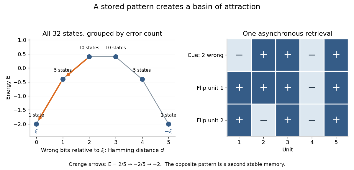
An exact five-unit memory landscape and correction of two wrong bits
. Each point represents every state at the indicated Hamming distance; multiplicities count the states. Arrows follow two actual updates of the illustrated cue under asynchronous Hopfield energy descent. This is an original finite calculation. Details.
Two-carrier Hall coefficient Created 2026-10-18 Updated 2026-10-20
For isotropic electrons and electron holes with positive mobilities, adding their weak-field electrical conductivity tensors and imposing zero transverse total current givesThe Hall coefficient changes sign at . Carrier abundance alone does not fix the sign; mobilities enter quadratically. The formula assumes , , independent semiclassical carriers, and no anomalous Hall contribution.
Hall carrier count versus valence Created 2026-10-18 Updated 2026-10-20
In a one-carrier isotropic Drude model, and an inferred carrier density is . Dividing by the atomic number density gives an effective Hall count per atom. A noninteger result need not mean a literal fractional count of valence electrons: multiple energy bands, anisotropic Fermi surfaces and different charge carrier mobilities can change the Hall coefficient. In a two-carrier isotropic approximation,Its sign identifies the dominant Hall response rather than necessarily the most numerous charge carrier.
Third-order dispersion 2026-10-18
The cubic term in a component's spectral phase, conventionally written , where is an angular frequency offset.
Plus-polarized gravitational wave Created 2026-10-18 Updated 2026-10-25
The measuring electric current crosses the layer planes. This geometry motivates the serial-layer paths in the two-current resistor model. A quantitative material calculation can also require interface electrical resistances, spin relaxation and spin accumulation; the circuit below intentionally isolates a smaller set of assumptions.
Current-in-plane magnetoresistance 2026-10-18
The measuring electric current flows along the layer planes. This is the geometry of the Fe-Cr giant magnetoresistance experiments. Scattering and current paths through an extended stack require a transport description; treating successive layers as ordinary series resistors would not follow from this geometry.
There are unlisted articles, also show them or only show them.