
Bosonic coincidence enhancement in two orthogonal orbitals Created 2026-10-18 Updated 2026-11-05
Place one noninteracting spin-zero boson in each of two orthonormal orbitals . Its normalized symmetric spatial wavefunction is . At coincident positions the probability density is , twice the labelled distinguishable-product value. Coincidence at an exact point is understood as a density or the limit of small detector volumes. If both particles occupy the same orbital, the normalized product is already symmetric and this comparison gives factor one instead; the factor two is not a universal property of every two-boson state.
Condensate fraction Created 2026-10-18 Updated 2026-11-05
The condensate fraction is the population of a macroscopically occupied one-particle state divided by the total particle number . For an interacting system, use a macroscopic eigenvalue of the one-particle density matrix, rather than assume that the relevant mode is an undeformed single-particle trap ground state. The condensate fraction is not generally the fraction measured as superfluid by a flow or rotation response.
For a harmonic function between and , , in bipolar coordinates, suppose and . Write the periodic boundary values as a Fourier seriesSeparation of variables givesEach radial factor solves and has endpoint values zero and one; the mean mode solves . Sufficiently regular boundary data give the required Fourier series solution. Uniqueness follows from the maximum principle for a harmonic function with zero Dirichlet boundary conditions on both circles. The formula follows the coordinate values; is the geometrically smaller circle.
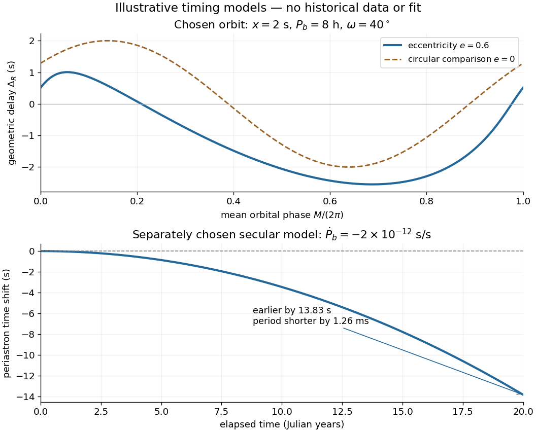
A tiny orbital period change accumulates into a larger timing shift. Choose the original model , with and . Expanding the accumulated cycle count givesNegative means an event of fixed orbital cycle count arrives earlier than a constant-period prediction. After twenty Julian years, the chosen period has decreased by , while the accumulated event shift is about . This is a time shift of periapsis passage; it is different from a rotation of the direction of periapsis.

David Gross and Frank Wilczek, and independently H. David Politzer, published their one-loop order Non-Abelian gauge theory results in adjacent 1973 Physical Review Letters papers. Both established a high-energy route to weak coupling; extrapolating into the low-energy region was a separate dynamical problem.[ref]
Ultraviolet Behavior of Non-Abelian Gauge Theories by David J. Gross and Frank Wilczek. 1973, p. 1345, acknowledgment of the independent calculation
[ref]Reliable Perturbative Results for Strong Interactions? by Hugh David Politzer. 1973, p. 1348, low-energy hypotheses versus the asymptotic result
The three shared the 2004 Nobel Prize in Physics for discovering asymptotic freedom in the theory of the strong interaction. David Gross's Nobel lecture describes the unexpected sign and their comparison of independent calculations.[ref]
The discovery of asymptotic freedom and the emergence of QCD by David J. Gross. 2005 reprint, p. 837, award footnote; p. 843, discovery narrative
In his lecture The Dilemma of Attribution, H. David Politzer emphasizes that the prize marks a wider community's work and that a tidy prize-centered history hides how discovery actually proceeds.[ref]The 1969 SLAC-MIT deep inelastic electron scattering experiment found approximate Bjorken scaling: an estimated deep-inelastic structure function depended mainly on a ratio of kinematic variables. Its restricted angular coverage did not separately determine both deep-inelastic structure functions, and the extraction assumed transverse virtual photons. This was motivation for a microscopic theory, not already a measurement of the QCD coupling.[ref]
Observed Behavior of Highly Inelastic Electron-Proton Scattering by M. Breidenbach and others. Printed p. 935, abstract; the stated transverse-photon assumption and limited separation of W1 and W2
The 1973 David Gross–Frank Wilczek calculation supplied a quantum field theory explanation of approximately free partons with calculable logarithmic corrections. Asymptotic freedom therefore permits approximate Bjorken scaling without requiring exact scale independence. The QCD coupling governs the corrections, while parton distribution functions and their evolution connect the short-distance calculation to a proton.[ref]
In a later direct test, H1 collided Positrons and protons at HERA and selected deep inelastic scattering events. A liquid-argon particle calorimeter identified the outgoing Positron with an associated track; calorimeter deposits and charged tracks reconstructed particle jets in the Breit frame. Vertex, timing and longitudinal energy-balance cuts suppressed backgrounds; two simulations checked detector corrections. Fits of particle jet cross sections to next-to-leading-order QCD extracted in transverse-energy bins, consistent with decreasing QCD coupling. Hadronization, parton distribution functions and renormalization scale choices limited the inference. This measures rates and fits a coupling, rather than directly reading a force meter.[ref]
Calibrated one-loop QCD evolution 2026-10-18
A useful original example fixes five active quark flavors and chooses and . These are illustrative inputs, not a measured determination. Integrating with givesConsequently , , and . Substituting returns the input, while differentiating returns the stated beta function. Rescaling all dimensional inputs by the same factor leaves the QCD coupling unchanged: only ratios enter. The reciprocal QCD coupling is a straight line against , so the calibration sets the intercept and sets the slope.
Changing the physical probe energy and changing an auxiliary renormalization scale are different operations. To isolate the latter, hold a hypothetical hard scale fixed and define , , and the toy approximationsUsing the one-loop order equation givesThe explicit logarithm cancels the order- scale drift. At , respectively, , whereas . These are values of an invented dimensionless observable chosen to expose the cancellation; they are not a cross section prediction. Smaller residual scale variation does not bound the unknown constant at the next loop order.
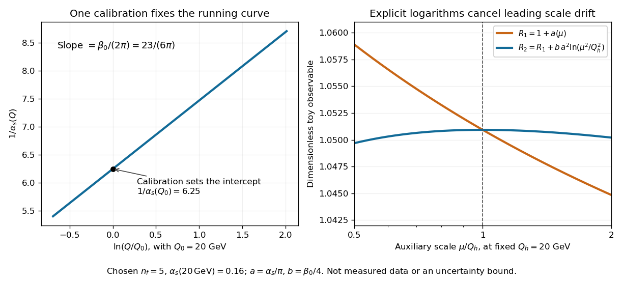
Calibrating a running coupling and cancelling leading auxiliary-scale dependence
. Left: the original five-quark flavor calibration written as an inverse QCD coupling. Right: varying the renormalization scale at fixed in the original toy . The reduced variation illustrates cancellation between running and an explicit logarithm; it is not an experimental uncertainty band. Details.
One-loop QCD antiscreening 2026-10-18
The contribution to is the net Non-Abelian gauge theory contribution; the term comes from quark loops. Thus quarks screen color charge, opposing asymptotic freedom. It is the net gluon contribution that produces antiscreening: the inferred QCD coupling decreases toward shorter distances. Unlike the electrically neutral photon, a gluon carries color charge and has self-interactions. Describing this as vacuum polarization must not imply that all vacuum contributions have the screening sign of quantum electrodynamics.[ref]
The discovery of asymptotic freedom and the emergence of QCD by David J. Gross. 2005 reprint, pp. 843–844, magnetic-response explanation; Eqs. 1–3
Individual gauge-dependent Feynman diagrams do not separately define observable screening clouds. A proof of the coefficient sums the gauge fixing, Faddeev-Popov ghost and matter contributions and extracts the charge renormalization; the final one-loop order coefficient is independent of the gauge choice. The beta function is negative near zero for integer . This is a statement about weak coupling, not a determination of the low-energy particle spectrum.[ref]
Reliable Perturbative Results for Strong Interactions? by Hugh David Politzer. 1973, pp. 1347–1348, Eqs. 3–7; warning below Eq. 7
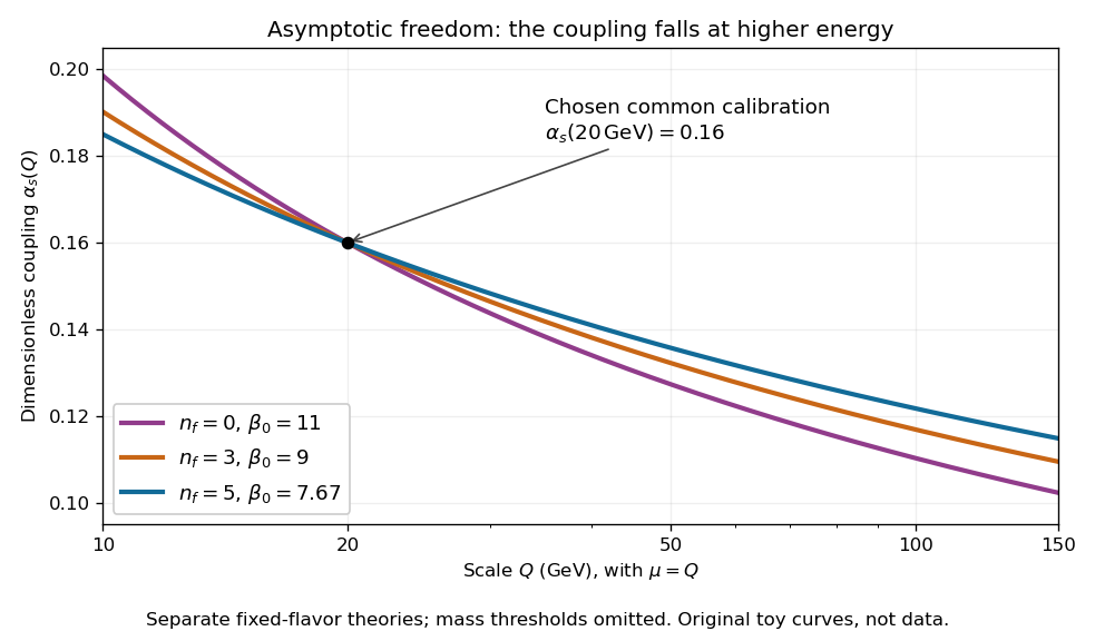
One-loop running couplings with a common chosen calibration
. Original fixed-quark flavor calculations with in each theory. More quark flavors reduce and slow the decrease at higher energy. The three curves have different strong-coupling scales; they are not successive threshold intervals of one physical theory. Details.
For an orbit of radius in the plane, . In spherical coordinates, at angle from the orbit normal, . The acceleration covariance in nonrelativistic radiation therefore gives the displayed pattern. Its axial power per solid angle is twice its equatorial value; no observation direction has zero time-averaged power. Integrating gives . The condition is essential: relativistic synchrotron radiation has a different beamed pattern.
The angular distribution of electric dipole radiation measures squared projections of the dipole axis, so a few intensity measurements need not determine that axis or the total radiated power uniquely. For a real unit dipole axis , the radiation-zone formula is . Equal intensities along , and permit four axes, up to reversal:Three generally different radiated powers are compatible with the same intensity data. Additional directional measurements or polarization information can remove the ambiguity.
For a concrete independent example, stipulate perpendicular motion, with the elementary charge, uniform magnetic field , incoming gyroradius and outgoing gyroradius . These are invented teaching inputs. Converting SI momentum to electronvolt units givesso and . Both a Positron and a proton with these momenta trace the same ideal arcs. Their kinetic energies differ because the relativistic energy-momentum relation givesThe second expression avoids subtracting nearly equal quantities when . For this calculation stipulate rounded rest energies and . The Positron interpretation gives and ; the proton interpretation gives only and . The corresponding proposed losses of kinetic energy are about and .
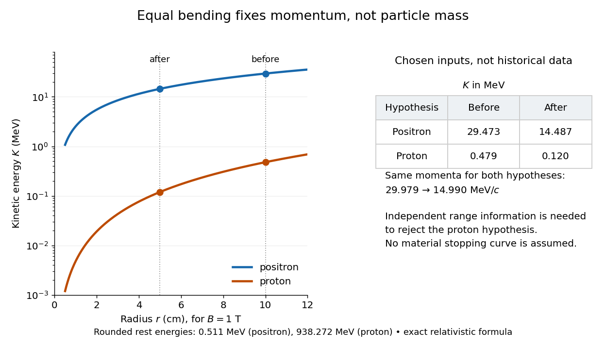

The small proton kinetic energy follows from , whereas here the Positron has and . Consequently magnetic bending alone cannot reject the proton. One needs an independent material constraint: could a proton at the proposed kinetic energy penetrate the plate and then travel at least the observed visible distance in the specified gas? A particle range shorter than that visible distance contradicts the hypothesis. The visible track need not include the stopping point: it already supplies a lower bound on particle range. No numerical particle range is assigned to this teaching example; that would require stopping data for the actual material and gas conditions. The experimental insight is to combine a geometric momentum measurement with an independent test of penetration.
Charge-sign ambiguity of a curved track Created 2026-10-18 Updated 2026-10-20
A photograph records a path but supplies no arrow of time. The Lorentz force depends on : reversing both electric charge and direction of travel leaves the spatial bending compatible with the same path. Thus a particular arc can represent a Positron travelling one way or an electron travelling the other. Knowing the magnetic field's polarity is necessary but insufficient. Gravity does not justify assuming that every cosmic ray track travels downward.
The lead plate adds a physical ordering. For a single particle crossing a passive absorber without an accelerating interaction, the outgoing momentum is smaller, so the outgoing gyroradius is smaller in the same magnetic field. The less curved segment comes first. Once this direction is assigned, the cross product in the Lorentz force determines the sign of electric charge. For the convention below, points out of the page; at upward velocity , . Bending to the right therefore means positive electric charge.
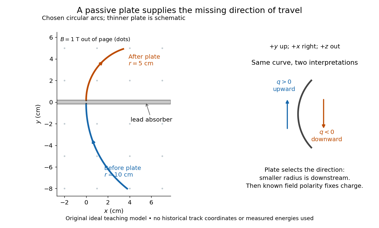

Magnetic forces do no work: the change of kinetic energy occurs through interaction with the material, not through the bending magnetic field. The ideal construction suppresses multiple scattering, kinetic energy fluctuations, and loss of kinetic energy in the gas. In an actual analysis one compares arcs away from the plate and allows a change of tangent from multiple scattering; one cannot interpret every kink as a change of electric charge. Short visible arcs, uncertain projection and small bending also limit a determination of magnetic rigidity.
Strong-bond limit of the alternating-spring chain Created 2026-10-18 Updated 2026-11-05
Take equal masses , atomic spacing , and alternating springs . The primitive unit cell contains a strong-bonded pair, so its length is and the Brillouin zone ends at . Expanding the exact alternating-spring chain dispersion relation givesThe low-frequency acoustic phonon branch moves almost rigid dimers of mass coupled by weak springs; its speed of sound tends to . The high-frequency optical phonon branch describes internal dimer stretch. At the zone edge the exact frequencies are and .
Rigid-motion zero modes of a spring framework Created 2026-10-18 Updated 2026-11-05
For unstressed central Hookean springs, the quadratic elastic energy is , with unit edge direction . A common translation gives zero displacement difference. An infinitesimal rotation also gives zero extension because a vector is perpendicular to its cross product with . Thus a noncollinear three-dimensional free framework has three translational and three rotational zero modes. Extra mechanisms can give additional zero modes; six is a lower bound until rigidity is established.
X-ray spectral attenuation operator 2026-10-18
For a fixed homogeneous absorber in a narrow-beam geometry, define the X-ray spectral attenuation operator on L1 space over a bounded positive energy interval. A physical input is an integrable function giving incident photon rate density. Let its linear attenuation coefficient be a measurable function, with . The transmitted uncollided density isHere is a fixed bounded detector response described by a measurable function; background has been subtracted. This is a positive linear operator on L1 space. Since , it cannot increase the integrated absolute incident rate. Multiplication of exponentials proves for successive layers of the same material. Ignore secondary radiation entering the detector, saturation and changes to the source. Discrete spectral lines use the finite-sum version below instead of an ordinary rate density.
For a chosen filter, stipulate , and input line rates in a common arbitrary rate unit. Assume equal calibrated detector weight for both lines. At ,The selected line's fraction rises from to , but its absolute rate falls by about . Filtering improves purity at the cost of signal. It multiplies existing components and cannot create a new emitted spectral line.
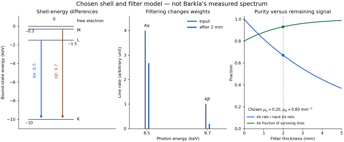

With just one integrated reading, , the two unknown line rates are underdetermined. If the source is unchanged between an empty-path reading and a filtered reading, the ideal inverse problem becomesThe determinant is nonzero, so these two ideal readings determine the two stipulated line rates uniquely. Identical coefficients would give zero determinant and destroy that separation. This small linear algebra example explains why absorber contrast supplies information, while also showing its limit: unknown scattered components or unknown detector weights add unknowns that two readings cannot determine.
Precision X-ray emission spectroscopy turns closely spaced spectral lines into quantitative constraints on atomic energy levels. Bragg's law makes a crystal an angular ruler for wavelength: resolving nearby directions can reveal components hidden inside an apparently single line. Accurate line positions and the ability to separate two lines are related, but distinct, experimental achievements.
Karl Manne Georg Siegbahn received the 1924 Nobel Prize in Physics; his lecture was delivered on 11 December 1925.[ref]
The X-ray Spectra and the Structure of the Atoms by Karl Manne Georg Siegbahn. Nobel Lectures, Physics 1922–1941; The X-ray Spectra and the Structure of the Atoms, heading, printed p. 81
His son Kai Siegbahn received the 1981 Nobel Prize in Physics for electron spectroscopy.[ref]
Facts on the Nobel Prize in Physics by Nobel Prize Outreach. Family Nobel Prize laureates in physics, Father and son: Manne and Kai Siegbahn
The Barkla characteristic X-ray experiment distinguished element-dependent K and L groups through absorption and excitation. Moseley's law related corresponding line frequencies across chemical elements to atomic number. Measuring the components within those groups asks a further question: which distinct atomic energy differences produce the neighbouring spectral lines?
Siegbahn's lecture organizes measured spectral lines into energy levels and resolved double levels.[ref]
The X-ray Spectra and the Structure of the Atoms by Karl Manne Georg Siegbahn. Nobel Lectures, Physics 1922–1941; Printed pp. 84–86, Figs. 1–2
The payoff is a map of atomic energy differences as well as an element's position in the periodic table. Barkla characteristic X-ray experiment 2026-10-18
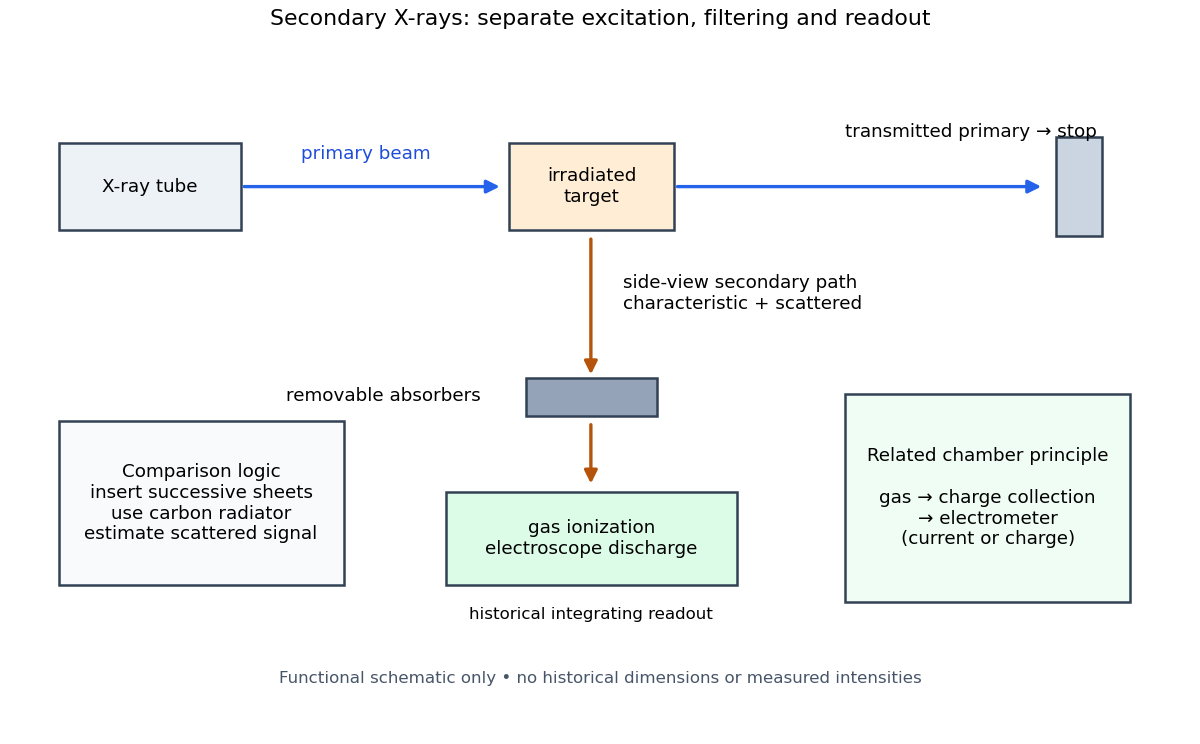
Charles Glover Barkla's 1911 paper describes irradiating a target with an X-ray tube and observing secondary X-rays using an electroscope. For soft Characteristic X-rays from tin, he used a soft primary beam and placed the electroscope close to the target to limit loss in air. Successive aluminium absorbers changed the gas-ionization signal. Thick absorbers suppressed the soft component; a carbon radiator supplied a comparison for the surviving scattered component. Subtracting this estimated contribution left approximately equal fractional losses through successive sheets, evidence for a nearly homogeneous component. Changing primary-beam hardness could suppress excitation of the more penetrating characteristic component.[ref]
The Spectra of the Fluorescent Röntgen Radiations by Charles Glover Barkla. Barkla, The spectra of the fluorescent Röntgen radiations (1911), p. 396: soft tube, nearby electroscope, aluminium sheets, carbon comparison and subtraction
An electroscope reads loss of stored electric charge; ionization in its detecting gas enables discharge. An ionization chamber with an electrometer instead measures the collected electric charge or electric current. These are integrating readouts: neither directly assigns an energy to each arriving photon. The diagram separates these functions without claiming a surviving apparatus drawing.

The K and L components were distinguished by their penetrating power and dependence on the emitting chemical element. Barkla's Nobel lecture, delivered on 3 June 1920 for the 1917 prize, explains that absorber-defined K radiation had seemed homogeneous, whereas later diffraction experiments resolved neighbouring spectral lines in both K and L groups. Absorber tests therefore distinguished groups without resolving every line.[ref]
Characteristic Röntgen Radiation by Charles Glover Barkla. Nobel Lectures, Physics 1901–1921; Barkla, Characteristic Röntgen radiation, printed pp. 392 and 395, PDF pp. 132 and 135: lecture date and limitations of absorption analysis
Henry Gwyn Jeffreys Moseley subsequently related the frequencies of corresponding spectral lines to atomic number. The approximate relation , with series-dependent constants , is Moseley's law; its discovery should be distinguished from Barkla's identification of characteristic secondary radiation.[ref]
Moseley and X Rays by University of Oxford Department of Physics. University of Oxford Department of Physics, Moseley and X rays: Moseley's graph and the story of Moseley and X-rays
A continuous incident frequency spectrum can contribute a continuous scattered background alongside discrete Characteristic X-rays. Here “scattered” identifies a production process, not a universal spectral shape: scattering of a narrow incident line need not make a continuum. In particular, the characteristic component is photon emission after vacancy creation, rather than simply the primary beam redirected. Source hardness, target substitution and absorber thickness probe different parts of that distinction. A surviving signal alone establishes neither an additional electron shell nor a fully resolved spectral line.
Grand-canonical Hamiltonian of a Bose field Created 2026-10-18 Updated 2026-11-05
For a repulsive contact-interacting Bose-Einstein condensate, the classical Hamiltonian density generating evolution in a frame rotating at the chemical potential is . Its integral is the grand canonical ensemble generator , not the physical energy alone. For the uniform mean-field theory minima satisfy , with a freely chosen constant phase. In the physical frame, the corresponding field has time factor .
Quadratic condensate fluctuation Lagrangian Created 2026-10-18 Updated 2026-10-20
Expand a repulsive Bose-Einstein condensate around the real uniform saddle as . After removing a constant and a temporal boundary term, the quadratic Lagrangian density is the displayed expression. Its equation mixes a fluctuation and its complex conjugate. Writing gives canonically paired amplitude and phase fluctuations and one positive Bogoliubov quasiparticle dispersion branch, with . The phase direction is a Goldstone mode; its zero uniform restoring force does not produce a second independent positive-frequency amplitude branch in this first-order-in-time theory.
For the faces of a closed polyhedron, take outward unit normal vectors. Applying the divergence theorem to an arbitrary constant vector field givesSince is arbitrary, the vector areas sum to zero. This is an oriented statement; the positive scalar surface areas do not cancel. The same proof works for every piecewise smooth closed boundary to which the divergence theorem applies.
There are unlisted articles, also show them or only show them.