
Pure positive operator-valued measure 2026-10-14
A POVM whose nonzero effects have rank one, , with normalized pure states and . Completeness is . This use of pure concerns effect rank, and does not mean an extremal point in the convex set of all POVMs.
POVM–ensemble duality for the maximally mixed state Created 2026-10-14 Updated 2026-10-20
A POVM in dimension corresponds to a quantum state ensemble with and , omitting zero effects. Its average is the maximally mixed state . Conversely any ensemble with that average defines a POVM by . These transformations are inverse. A pure POVM corresponds exactly to a pure-state ensemble decomposition of .
For a bounded real linear functional on the space of continuous functions on a compact space, define for . The decomposition for proves additivity on the positive cone; positive homogeneity is immediate. Extend by differences, and put . Both are positive linear functionals. Their norms sum to , using the substitution .
For a slender porous thermal plume, Darcy law gives , with . If and is the conserved excess convective heat flux per span, then the kinematic momentum flux is , and the buoyancy flux is . The hyperbolic-secant porous plume profile has . Multiplication of and by gives physical mass flux and the density-weighted Darcy second moment. Intrinsic pore-velocity momentum flux instead has an additional inverse-porosity factor. Momentum conservation here follows from the heat/velocity proportionality, not from an inertia balance: porous drag balances buoyancy locally.
Compact radial cubic-diffusion profile 2026-10-14
Spherical nonlinear-diffusion source profile Created 2026-10-14 Updated 2026-10-31
For in three dimensions and total mass , the nonnegative radial source solution is , with . Integrating the similarity equation once gives , and normalization fixes the compact-support radius. The flux vanishes at the moving front, so the profile solves the equation weakly and approaches the prescribed point mass as time tends to zero.
Surface sound speed of a polytropic star 2026-10-14
In a plane-parallel polytropic atmosphere of index , let measure depth from a zero-pressure boundary and take constant gravitational acceleration . The stellar hydrostatic equation and integrate to . Consequently the adiabatic sound speed satisfies , so . This local relation does not justify extrapolating a surface model to the stellar core.
Latent-heat polynya 2026-10-14
A latent-heat polynya remains relatively open because winds or currents remove newly formed sea ice. Sustained cooling can produce large amounts of ice even while local ice concentration remains low. Opening is maintained by export, not by latent heat warming the ocean enough to prevent freezing.
Sensible-heat polynya 2026-10-14
A sensible-heat polynya is maintained by ocean heat delivered through currents, mixing or upwelling, sufficient to inhibit local sea ice growth. Mechanical export and sensible heating may act together, so this classification identifies a dominant mechanism rather than an exclusive geographical class.
Northeast Water Polynya 2026-10-14
The Northeast Water Polynya is a recurrent open-water region off northeast Greenland. Ice barriers, local currents and winds organize ice divergence; summer opening and winter new-ice export need not have the same dominant forcing. Its regional northward coastal flow must not be confused with assuming that every current along east Greenland flows southward.
North Water Polynya 2026-10-14
The North Water Polynya, also called Pikialasorsuaq, lies between northern Greenland and the Canadian Arctic in the Smith Sound and northern Baffin Bay region. An upstream ice arch can restrict replenishment of drifting Arctic ice while winds and currents export newly formed ice. Ocean heat contributes in some parts of the polynya.
Pease polynya model 2026-10-14
The simplest Pease polynya model balances offshore ice export at speed against production of new ice at thickness rate within an open strip of width . Newly formed ice is collected into an edge of prescribed thickness , with negligible residence time. Per unit coastline length, conservation gives . For constant positive parameters,Thus the equilibrium width is and the relaxation time is . If warming reduces while stay fixed, both increase. With the positive-freezing equilibrium ceases to apply. Finite frazil ice residence, variable atmospheric forcing and alongshore transport require extensions of the model.
Dilute frazil polynya similarity solution Created 2026-10-14 Updated 2026-11-05
This reduced polynya model describes a wind-driven, nearly uniform surface layer containing dilute frazil ice. Let be distance from the opening, the layer depth, its horizontal speed, and its ice volume fraction. Use reference liquid mass density except in buoyancy, where is the liquid-minus-ice mass density difference. Let be the uniform wind shear stress and the atmospheric cooling heat flux divided by .
For a linear liquidus , far-field salinity , specific heat capacity and specific latent heat , define , and . The extra sensible term in accounts for the cooling associated with salt enrichment. The chosen depth-averaged momentum, ice-production and buoyancy balances areTheir numerical coefficients belong to this particular layer closure. The first two give and . Seeking a similarity solution with gives ; substitution into the third balance yieldsThus layer depth, speed and retained ice fraction all grow as . The increasing eventually violates the dilute approximation. If crystals are exported out of the layer, their enthalpy and ice-volume flux must be included through the frazil export enthalpy balance; retained fraction is not automatically total production.
There is a sequence of complex polynomials converging pointwise on the whole plane to the sign of the imaginary part, with value zero on the real axis. For each , take the compact union of the upper rectangle , its lower reflection and the real segment . Its complement is connected. The function equal to one, minus one and zero on disjoint neighborhoods of the three components is holomorphic. The polynomial Runge theorem provides a polynomial within of it on the union. Every fixed point lies in its corresponding component for all large , proving pointwise convergence. The limit is discontinuous, so the convergence cannot be locally uniform near the real axis. This illustrates how pointwise approximation by holomorphic functions differs from locally uniform approximation.
Runge exhaustion of a slit disk 2026-10-14
For the unit disk with the nonpositive real radius removed, compact sets , , exhaust the domain. Each has connected complement: its inner and outer complementary regions join through the missing angular sector. The polynomial Runge theorem gives a polynomial within of a given holomorphic function on . Every compact subset lies in some , so these polynomials converge uniformly on compact subsets.
Lagrange polynomial 2026-10-14
The Lagrange polynomial writes the interpolation polynomial as a linear combination of Lagrange cardinal polynomials. Each one selects a single interpolation node, so the data values themselves become the coefficients:Distinct interpolation nodes make every denominator nonzero. At , all terms vanish except . This gives an explicit construction without solving for monomial coefficients. The elegance of the Lagrange polynomial is that it builds all constraints into the basis, leaving no equations to solve for the data values.
For and , substitution givesAt , the Lagrange cardinal polynomial values are , so . A negative Lagrange cardinal polynomial value is allowed: these weights sum to one but need not be probabilities.
The product form is especially useful for deriving differentiation weights from nodal evaluations and quadrature rules. For repeated numerical evaluation, the barycentric interpolation formula reorganizes the same Lagrange polynomial into precomputed weights and sums; it avoids evaluating every full product at every argument.
Runge's phenomenon 2026-10-14
The Runge phenomenon is the failure of increasing-degree polynomial interpolation at equally spaced interpolation nodes to converge to some smooth target functions, with large oscillations near the ends of the interval. It is a property of the approximation problem, and can occur even with exact arithmetic. A numerically stable evaluation method cannot remove it. Endpoint clustering, as in Chebyshev-Lobatto nodes, changes the approximation problem and can greatly improve it.[ref]
https://fncbook.com/python/stability-1/. Driscoll and Braun, Fundamentals of Numerical Computation, §9.3.1–9.3.2
Take on and polynomial degree at most . Use either or for . Each interpolation polynomial passes through all eleven of its own samples, yet the first has severe endpoint oscillations and the second stays much closer to the target function. Evaluating both by the barycentric interpolation formula on equally spaced points, including the endpoints, gives sampled maximum absolute errors of approximately and , respectively: about a -fold reduction. These are maxima over the stated grid, not certified maxima over the continuous interval. The generator separately checks exact reproduction of all stored nodal values.
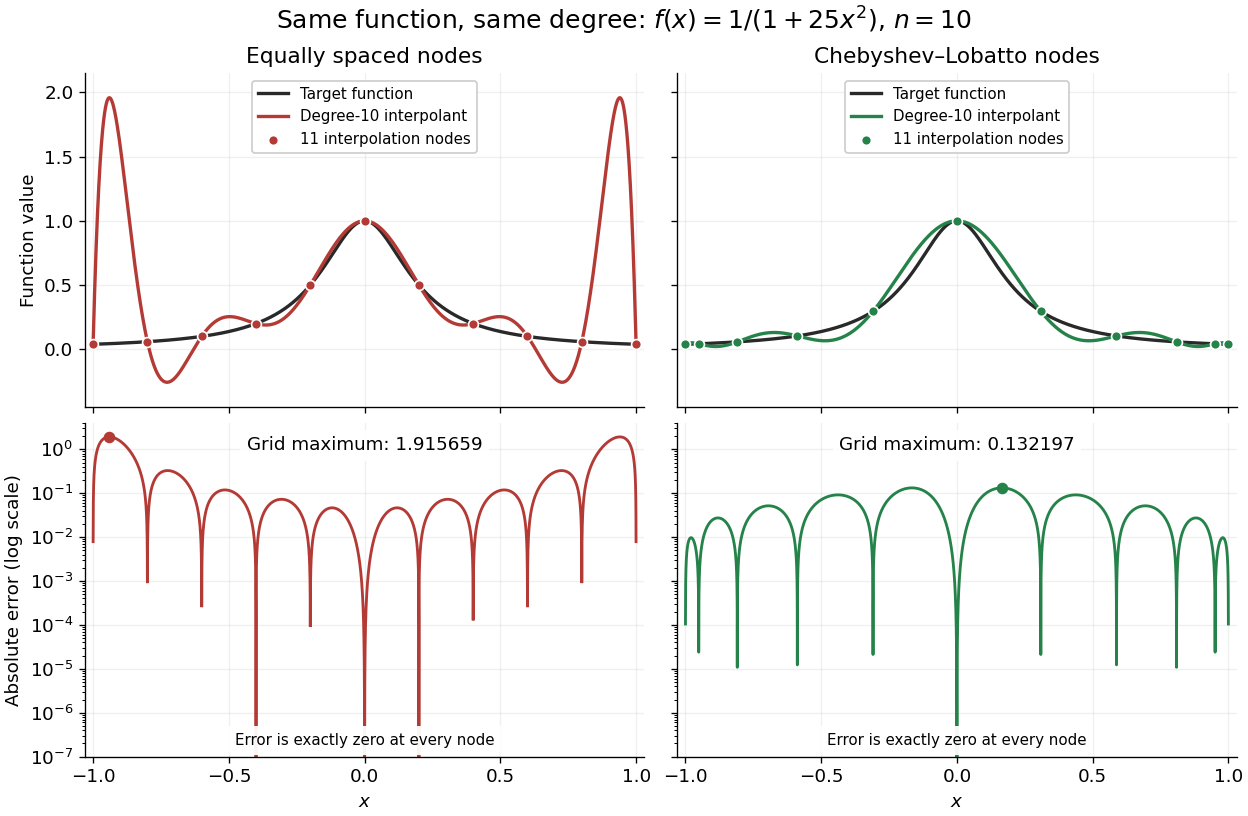
Degree-10 interpolation of the Runge function at equally spaced and Chebyshev-Lobatto nodes, with absolute errors
. Details. 
The polynomial interpolation error formula explains why interpolation nodes enter the analysis. If has continuous derivatives on an interval containing and all the interpolation nodes, then for a suitable in that interval,At an interpolation node the error is zero directly. Away from the interpolation nodes, both the product and the high-order derivative matter. A short proof applies Rolle's theorem repeatedly to , which vanishes at distinct points.[ref]
https://fncbook.com/polynomial/. Driscoll and Braun, Fundamentals of Numerical Computation, §9.1.2, Theorem 9.1.3
The successful comparison here does not assert that Chebyshev-Lobatto nodes solve every approximation problem for every function. The derivatives, the polynomial degree, and measurement errors still matter. The Lebesgue constant of interpolation measures worst-case amplification of nodal errors, while the polynomial reproduction error bound relates interpolation to the best uniform approximation available at that polynomial degree.
For a real continuous function on a compact interval, choose its best uniform approximation of polynomial degree at most . If its error is nonzero, the Chebyshev alternation theorem supplies ordered alternating extrema. The intermediate value theorem gives a zero of in each intervening interval. At these distinct points, the polynomial interpolant is exactly . If the best error is zero, arbitrary distinct nodes suffice. The Weierstrass approximation theorem shows that these function-dependent interpolants converge uniformly. The nodes depend on the target function; the conclusion does not provide one universal node sequence for every continuous target.
Interpolation polynomial Created 2026-10-14 Updated 2026-10-20
An interpolation polynomial for distinct nodes and prescribed values is a polynomial satisfying . There is a unique such polynomial of degree at most : the Lagrange interpolation polynomial constructs it explicitly, and uniqueness follows because a nonzero degree-at-most- difference cannot have distinct roots. Newton interpolation polynomials express the same object using divided differences.
Poly-infinite cyclic group Created 2026-10-14 Updated 2026-11-05
A poly-infinite cyclic group has a finite subnormal series all of whose nontrivial factors are infinite cyclic groups. Intersecting its series with a subgroup again gives trivial or infinite cyclic factors; repetitions may be deleted. Splicing a kernel series with the preimage of a quotient series proves closure under extensions. Such groups are finitely presented groups: induct on the series, split the last extension by an infinite cyclic quotient, and use finite presentation of a semidirect product.
There are unlisted articles, also show them or only show them.