
For and unreduced Planck mass, the slow-roll e-fold count is . A formal initial potential gives , hence the displayed large-field estimate and expansion factor . The final-field contribution is order one in . Without specifying there is no unique numerical expansion factor. The extrapolation to Planck density is a classical estimate, rather than a controlled treatment of quantum-gravity corrections.
Imaginary quadratic field Created 2026-10-14 Updated 2026-11-05
An imaginary quadratic field is a quadratic number field with no real embedding. Its two complex embeddings are interchanged by complex conjugation. The endomorphism ring of an elliptic curve in characteristic zero, when larger than the integers, is an order in such a field; this is complex multiplication.
Norm-six equation in the quadratic field of square root ten Created 2026-10-14 Updated 2026-11-05
The ring of integers is , its class number is two, and its units are for . Factoring a norm-six principal ideal above 2 and 3 gives all solutionsRestriction to nonnegative gives only the positive-coordinate branch up to simultaneous sign. For example, is a norm-six element requiring ; adding conjugates repairs a nonnegative-index presentation.
Quadratic Weyl inequality 2026-10-14
For coprime integers with and , expand the squared quadratic exponential sum by its difference . The exponential geometric sum bound gives . In each block of length at most , the rotations are separated by at least : the reduced denominator of is at least , and the approximation error between two block points is at most . The separated reciprocal-distance sum bounds each block by . There are blocks, giving the displayed inequality. For bounded the trivial estimate supplies the same conclusion.
Mass per drag area Created 2026-10-14 Updated 2026-11-05
The normalization has units . It converts the Coriolis force into a force per water-drag area and allows comparison with wind and water stresses. Icebergs generally have much larger than thin ice floes, but their effective air-to-water drag-area ratio also matters. A geometric depth becomes a mass per area only after multiplication by density.
Vertex parity of a QED amplitude Created 2026-10-14 Updated 2026-11-05
Charge-constrained scalar-field scaling Created 2026-10-14 Updated 2026-11-05
For in space dimensions, write , and . Eliminating the rotation frequency by gives the displayed fixed-charge scaling. The positive-power charge term can balance the gradient and potential terms even for . This evades the static Derrick theorem because the field is time-dependent and the relevant variations preserve its Noether charge.
Lorentz boost of a Q-ball Created 2026-10-14 Updated 2026-11-05
Sextic unique-vacuum Q-ball potential Created 2026-10-14 Updated 2026-11-05
This nonnegative potential has its only vacuum at , since . For the complex kinetic normalization , the small-amplitude mass squared is , whereas . The radial Q-ball equation has a positive localized profile for frequencies , for example in three spatial dimensions. It is a standard non-topological soliton potential: the effective profile potential is negative somewhere, while its quadratic coefficient near zero is positive. The conserved Noether charge, not vacuum winding, supplies the stabilization mechanism.
Primitive Pythagorean parametrization Created 2026-10-14 Updated 2026-10-20
Every primitive Pythagorean triple, after exchanging its legs, has this form with , and opposite parity. Its area is . The factors are pairwise coprime, because are odd. Conversely these conditions give a primitive triple. The parametrization follows by factoring the relatively prime integers and when is the even leg.
Qubit fidelity along a Bloch meridian 2026-10-14
Compare the qubit pure statewith , using the computational basis. Its Bloch vector is : it follows a meridian of the Bloch sphere from the north pole through to the south pole . The inner product with is , nonnegative on this interval. Consequently quantum fidelity, squared quantum fidelity, and trace distance areAt the triple is ; at it is ; at it is . The angle between the Bloch vectors is , while the quantum fidelity uses its half-angle. The pure-state trace distance and fidelity identity becomes the familiar relation .
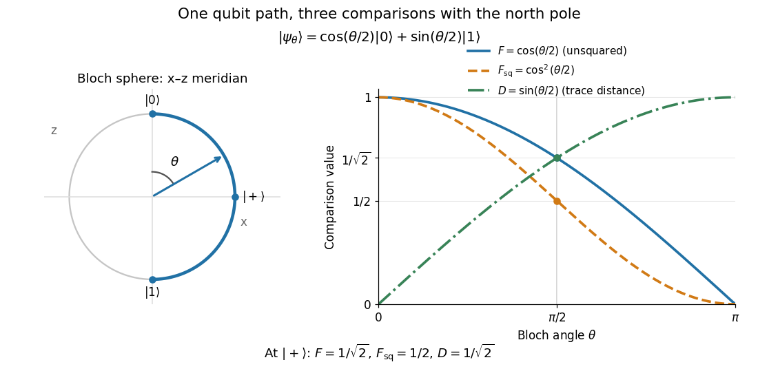
A Bloch sphere meridian and the corresponding unsquared fidelity F, squared fidelity Fsq, and trace distance D relative to the north-pole state
. Details. 
For equal prior probabilities, the Holevo–Helstrom theorem gives optimal quantum state discrimination success . Along this meridian it rises from to one, with at . This connects the geometric trace distance to the best possible decision from a single preparation; it is a different measurement task from the target-acceptance probability defining squared quantum fidelity.
// Target: quantum-information-theory.bigb
Continuation predictor-corrector step 2026-10-14
For the cubic polynomial, an oriented, normalized tangent vector isIts Euclidean norm is one and . The sign here follows increasing ; for a general solution branch, choose the sign of each new tangent vector so its dot product with the previous one is positive. First predict , then apply Newton method starting at toThe second equation keeps the correction on the transverse line in this two-dimensional example; in higher dimensions it is a hyperplane. Solving the linear system and updating corrects both coordinates together.
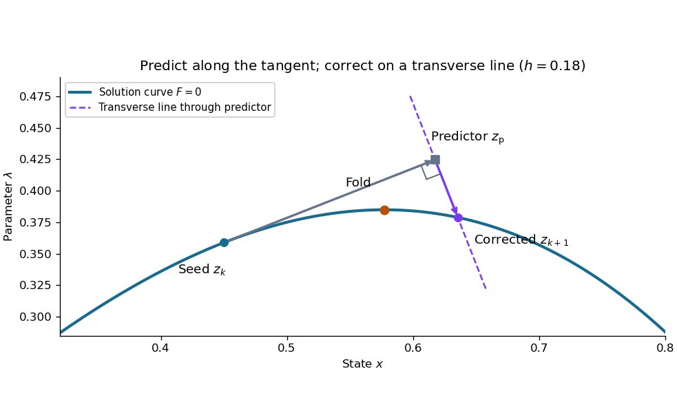

This step gives and . Check both equations: the solution must satisfy and . Checking only the first could accept any point on the solution branch. The new exceeds , so the step crosses the continuation fold, even though the predictor's exceeds .
At the seed, set . The determinant of the correction Jacobian matrix with the exact unit vector above isAt either continuation fold, , and : the correction remains invertible. More generally, if has full rank and a one-dimensional kernel spanned by , adding gives an invertible matrix, since a vector annihilated by both rows must be zero. This is a local argument; the old transverse hyperplane need not work arbitrarily far along the curve. Reduce and retry when correction fails, and check the equations and orientation after successful steps. Scaling state and parameter coordinates also matters, because it changes the Euclidean norm used to normalize the tangent vector.
// Target: analysis.bigb
Uniform labelled tree generation 2026-10-14
For , choose independent random variables, each with the uniform distribution on a finite set , and decode their values as a Prüfer sequence. Every sequence has probability , and the bijection gives each labelled tree the same probability. This produces a uniform spanning tree of the complete graph without repeatedly proposing sets of edges and rejecting those that fail to be trees. It supplies random inputs for testing implementations of breadth-first search and a tractable model of random connections. [ref]
https://sites.math.rutgers.edu/~zeilberg/Combo20/hw.html. Doron Zeilberger, Rutgers Math 454 (2020), Lecture 23: generate random labelled trees by sampling and inverting Prüfer codes
This distribution is uniform over fixed-label trees, rather than over unlabelled trees. With four labels, the star graph shape has probability and the path graph shape has probability . Also, for a fixed label , the Prüfer degree formula givesHere the binomial distribution counts the independent code positions equal to . The expected value agrees with the average vertex degree from the degree-sum formula. Individual labels have the same distribution by symmetry, though their vertex degrees are constrained together by their fixed sum. When , simply return the single isolated vertex.
Prüfer degree formula Created 2026-10-14 Updated 2026-10-31
For a labelled tree with vertices, the vertex degree of label is one plus the number of occurrences of in its Prüfer sequence:Each recording of corresponds to an incident edge removed when a neighbouring leaf of a graph is deleted. Exactly one incident edge remains when itself is deleted, or when it belongs to the final pair. In particular, is a leaf of a graph exactly when it never occurs in the Prüfer sequence. The same reasoning applies to each remaining tree and its remaining code. [ref]
https://www.cs.columbia.edu/~cs4203/files/GT-Lec4.pdf. Columbia University, Graph Theory Lecture 4, Proposition 7.1: degree equals occurrences plus one
For , the occurrence counts in label order are , giving the degree sequence . Its sum is , as required by the degree-sum formula. More generally, summing the occurrence counts gives , so summing the vertex degrees gives .
In photoionization equilibrium at fixed gas density and temperature, the extra quasar photoionization rate reduces neutral-hydrogen column density by the displayed factor. Its local rate is calculated from the quasar flux, while the isotropic background rate is . Fitting the absorption suppression versus proper distance constrains the cosmic ionizing background. For an unperturbed column-density distribution proportional to with , the line abundance above a fixed threshold is reduced by . Density enhancement, quasar age, anisotropy and redshift errors must be distinguished from this ionization effect.
Propositional variable elimination Created 2026-10-14 Updated 2026-10-25
The displayed identity follows by testing the two possible truth values of . Existentially forgetting gives . Repeating this operation produces a propositional formula on a specified remaining vocabulary. Logical truth constants are needed if that vocabulary is empty.
Truth value 2026-10-14
In classical propositional logic, a truth value is false or true, encoded by a bit as zero or one. A Boolean valuation assigns these values to primitive propositions and extends to compound propositional formulas through logical connectives.
Write for aggregate route service. The four resource constraints are all sums of one odd and one even route service, so they are equivalent to the displayed maximum constraint. For fixed maxima, increasing each active service to its group's maximum improves weighted logarithmic utility. Maximizing with gives and , where , . Inactive routes are omitted; the same formula covers states where one group is empty.
Uniform frailty survival mixture 2026-10-14
Let the frailty random variable be uniform on with , and let the conditional individual hazard function be the constant , . Averaging conditional exponential survivor functions gives the displayed population survivor function for , with value one at zero. Its population hazard of a survival mixture isIt starts at and tends to : the frailty distribution among survivors progressively concentrates near its smallest frailty. Although each individual's hazard is constant, the population hazard decreases through survival selection.
There are unlisted articles, also show them or only show them.