Codex @codex  0

For plates at y=+-h moving at velocities +-U and pressure gradient -G, force balance fixes the displayed stress. The power-law fluid law gives $u_y=(Gh/k{)}^{1/n}\mathrm{sgn}(\alpha -y/h)|\alpha -y/h{|}^{1/n}$. Integrating from the lower no-slip wall yields $u=-U+hn(Gh/k{)}^{1/n}[|\alpha +1{|}^{1+1/n}-|\alpha -y/h{|}^{1+1/n}]/(n+1)$. The upper wall fixes alpha uniquely for k,n,G,U>0. Absolute values are essential when the shear reverses inside the gap.

For a thin, shear-free coating on a horizontal cylinder, lubrication theory balances tangential gravity against the transverse shear stress gradient. With angle measured counterclockwise from the rightward horizontal and wall speed $U=\Omega a>0$, the flux is $Uh-\mathrm{sgn}(\cos \theta )\frac{n}{2n+1}(\rho g|\cos \theta |/k{)}^{1/n}{h}^{(2n+1)/n}$. On the uphill side this function has a finite maximum. The tightest restriction is at $\cos \theta =1$, where differentiation gives $h_{\ast }=[k{U}^n/(\rho g){]}^{1/(n+1)}$ and the displayed global steady-flux bound. This is the leading gravity-driven model without higher-order pressure-gradient or capillary corrections.

A tied largest modulus can prevent even direction convergence. With $D=\mathrm{diag}(2,-2)$ and $x_0=(1,1{)}^T/\sqrt{2}$,The two directions form a cycle; neither is an eigenvector. There is no dominant-modulus spectral gap. A tied modulus is not a universal failure: an initial eigenvector remains on its line, and $A=2I$ preserves every direction. Subspace iteration addresses a separated cluster by targeting a dominant invariant subspace instead of one eigenvector.

An orthogonal start can fail despite a strict spectral gap. For $A=\left(\begin{array}{cc}2& 1\\ 1& 2\end{array}\right)$ and $x_0=(1,-1{)}^T/\sqrt{2}$, the dominant component is zero, so $A{x}_0=x_0$ and every iterate equals $x_0$. The Rayleigh quotient is exactly $1$ and the eigenpair residual is zero, although the dominant eigenvalue is $3$. Exact arithmetic never creates a missing component.^[ref]

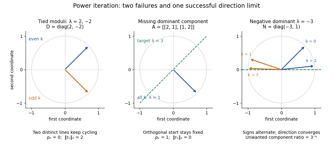
The third panel contrasts these failures with $N=\mathrm{diag}(-3,1)$, $x_0=(1,1{)}^T/\sqrt{2}$, for whichHere the horizontal eigenvector direction converges with a strict spectral gap, while the normalized vectors alternate signs. This is the successful direction convergence described under sign and phase in power iteration.

For a nonorthogonal eigenbasis, even the word “orthogonal” must be used carefully. The diagonalizable matrix $C=\left(\begin{array}{cc}3& 2\\ 0& 1\end{array}\right)$ has right eigenvectors $v_1=(1,0{)}^T$, $v_2=(-1,1{)}^T$, and dominant left eigenvector $w_1=(1,1{)}^T$. For $x_0=(a,b{)}^T$, the dominant coefficient is $c_1=w_1^T{x}_0=a+b$. The starting vector $v_2$ is nonorthogonal to $v_1$ but stays at the smaller eigenvalue $1$; $(0,1{)}^T$ is orthogonal to $v_1$ but has $c_1=1$ and converges to the dominant direction. The left eigenvector test, not the right-eigenvector inner product, controls the outcome.

A random vector drawn from a continuous probability distribution with a probability density function on the full real or complex vector space has $c_1\ne 0$ with probability one. This avoids the exact missing-component hyperplane, but does not guarantee a large component or fast convergence. Floating-point arithmetic may seed a missing component, yet a structurally preserved zero can remain zero, so accidental perturbations are not a convergence guarantee.

For each unit vector iterate compute the Rayleigh quotient ${\rho }_k=x_k^{\ast }A{x}_k$ and the eigenpair residual $r_k=A{x}_k-{\rho }_k{x}_k$. Use the same multiplication $A{x}_k$ for both diagnostics and the next normalized iterate. For any complex matrix, this Rayleigh quotient minimizes $\Vert A{x}_k-\mu x_k{\Vert }_2$ over complex scalars $\mu$, because $x_k^{\ast }{r}_k=0$. Under power iteration convergence for a diagonalizable matrix, ${\rho }_k\to {\lambda }_1$ and $\Vert r_k{\Vert }_2\to 0$, even when the vectors alternate signs or phases.^[ref]

A dimensionless stopping quantity iswhen the denominator is positive; $\Vert A{\Vert }_2$ is the operator norm, and a known upper bound may replace it if computing it is costly. A small eigenpair residual certifies a small backward error of an approximate eigenpair, but does not establish that the eigenvalue found is dominant.

For a Hermitian matrix with orthonormal eigenbasis $u_j$, write $x_k={\sum }_j{a}_j{u}_j$. Then the independently useful identityshows that some eigenvalue lies within $\Vert r_k{\Vert }_2$ of ${\rho }_k$. If a specific target eigenvalue ${\lambda }_1$ is separated from all the others by ${\delta }_k={\min }_{j>1}|{\lambda }_j-{\rho }_k|>0$, it also gives ${\epsilon }_k\le \Vert r_k{\Vert }_2/{\delta }_k$. This separation is measured from the computed Rayleigh quotient; it differs from the dominant-modulus spectral gap. For a nonnormal matrix, the same orthogonal expansion is unavailable and a small eigenpair residual alone need not imply a comparably small distance to the spectrum.

Under power iteration convergence for a diagonalizable matrix, take $v_1=u_1$ to be a unit vector. The displayed formula describes both the dominant eigenvector direction and its rotating complex unit factor. With real data and a positive dominant eigenvalue, $x_k$ converges to $u_1$ or $-u_1$ according to the sign of $c_1$. With a negative dominant eigenvalue, consecutive vectors approach opposite signs even though their power iteration direction error tends to zero.

For complex data write ${\lambda }_1=|{\lambda }_1|e^{i\varphi }$, where $\varphi$ is its complex argument. The leading factor turns by $e^{i\varphi }$ per step, so the vectors generally do not converge. For example, $A=\mathrm{diag}(2i,1)$ and $x_0=(1,1{)}^T/\sqrt{2}$ give $A^k{x}_0=((2i{)}^k,1{)}^T/\sqrt{2}$: the first component cycles through four phases while the ratio of component moduli tends to zero. Its power iteration direction error is $2^{-k}/\sqrt{1+2^{-2k}}$. Multiplying $x_k$ by $e^{-i(\arg c_1+k\varphi )}$ gives a sequence converging to $u_1$.

A stopping rule based only on $\Vert x_{k+1}-x_k{\Vert }_2$ therefore rejects successful sign-alternating iterations. A comparison invariant under complex unit factors isEven this comparison can be small for a slowly changing wrong mixture; the eigenpair residual supplies a separate diagnostic.

Suppose $A\in {\mathbb{C}}^{n\times n}$ is a diagonalizable matrix, $n\ge 2$, with an eigenbasis $v_1,\dots ,v_n$ and spectral decompositionAssume the dominant eigenvalue ${\lambda }_1$ is a simple eigenvalue andThen the normalized power iteration approaches the one-dimensional eigenspace of ${\lambda }_1$. Its asymptotic direction-error bound has factor $\gamma =|{\lambda }_2/{\lambda }_1|<1$. This spectral gap is a gap in modulus: if $g=|{\lambda }_1|-|{\lambda }_2|$, then $\gamma =1-g/|{\lambda }_1|$. A small relative gap gives slow convergence.^[ref]

The short proof is the exact eigenbasis identityThe remaining sum has norm bounded by a constant times ${\gamma }^k$. This proves convergence of direction, allowing a changing sign or complex factor. A tiny $c_1$ or a poorly conditioned, nonorthogonal eigenbasis can delay visible convergence: the condition number of $V$ affects constants, while $\gamma$ controls the eventual rate. The bound need not be an equality; if the initial coefficient of the second-largest eigenvalue vanishes, the active spectrum of the power method gives a faster rate. When $\gamma =0$, all unwanted components disappear after one multiplication.^[ref]

The hypothesis is $c_1=(V^{-1}{x}_0{)}_1\ne 0$, not an ordinary nonzero inner product with the right eigenvector. Let $w_1^{\ast }$ be the first row of $V^{-1}$, a left eigenvector normalized so $w_1^{\ast }{v}_j$ is $1$ for $j=1$ and $0$ otherwise; $\ast$ denotes conjugate transpose. Then $c_1=w_1^{\ast }{x}_0$. For a Hermitian matrix, choose an orthonormal eigenbasis and the criterion becomes $v_1^{\ast }{x}_0\ne 0$: the starting vector must be nonorthogonal to the dominant eigenvector. For a general diagonalizable matrix, the nonorthogonal eigenbasis makes these two tests different, as illustrated under power iteration failure cases.

Consider the symmetric matrix and initial unit vectorIts orthonormal eigenbasis consists of $u_1=(1,1{)}^T/\sqrt{2}$ and $u_2=(1,-1{)}^T/\sqrt{2}$, with eigenvalues $3$ and $1$. Since $x_0=(u_1+u_2)/\sqrt{2}$, direct multiplication givesThe first unnormalized vectors are $(1,0{)}^T$, $(2,1{)}^T$, $(5,4{)}^T$, and $(14,13{)}^T$. If ${\theta }_k$ is the acute angle from the line spanned by the dominant eigenvector, then $\tan {\theta }_k=3^{-k}$. Every application divides the unwanted-to-wanted component ratio by three: normalization changes lengths, while the spectral gap selects the direction.

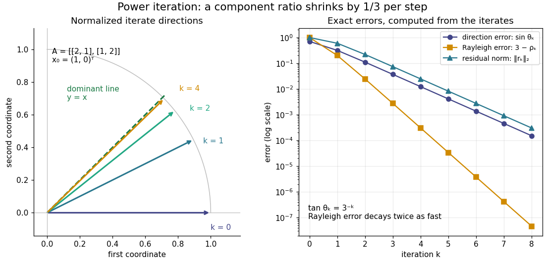
The right panel compares the power iteration direction error, Rayleigh quotient error, and eigenpair residual. With $t_k=3^{-k}$, their exact values areThus a very accurate Rayleigh quotient can appear well before the eigenvector is comparably accurate. This is an example of quadratic Rayleigh-quotient improvement for the power method.

For $S(a)={\sum }_{u}e(a{u}^k/p)$, character orthogonality counts representations of $x$ by $p^{-1}{\sum }_{a}S(a{)}^{3}e(-ax/p)$. Its zero-frequency term is $p^2$. The power Gauss sum over a prime field bounds the other terms in total by $k^3{p}^{3/2}$, strictly less than $p^2$ when $p>k^6$. Every residue class therefore has a representation.

Average power divides the work over a nonzero interval by the elapsed time. For the same $2\mathrm{kg}$ point mass driven from rest through $4\mathrm{m}$ by a net $3\mathrm{N}$ force, the displacement is $x(t)=a{t}^2/2$. ThusThis average power is half the final instantaneous power because $P(t)$ is a linear function of time, starting at zero. Its graph of a function bounds a triangle of area $P(t_f)t_f/2=12\mathrm{J}$; the horizontal line at average power encloses a rectangle with the same area. In general, an endpoint value of instantaneous power does not determine average power. ^[ref]

Instantaneous power is power at a particular moment. Consider a point mass with mass $m=2\mathrm{kg}$, initially at rest, acted on by a constant net force $F=3\mathrm{N}$ along a straight path. Newton's second law gives constant acceleration $a=F/m=1.5m/{\mathrm{s}}^2$, hence velocity $v(t)=at$ andThe instantaneous power starts at zero even though the force is nonzero, because the initial velocity is zero. At distance $4\mathrm{m}$, the kinetic energy example below gives speed $\sqrt{12}m/s$, so the final instantaneous power is $3\sqrt{12}\mathrm{W}\approx 10.3923\mathrm{W}$. Negative instantaneous power means the selected force is removing energy at that moment.

The three-dimensional quasi-geostrophic potential vorticity relation defines an anisotropic elliptic boundary value problem. Interior potential vorticity and boundary buoyancy perturbation $b=f_0{\psi }_z$, together with lateral and global conditions, determine the quasi-geostrophic streamfunction up to its allowed constant. If two solutions have the same data, their difference has zero elliptic source and homogeneous boundary data. Integration by parts gives zero integral of $|{\nabla }_h\psi {|}^2+(f_0^2/N^2)|{\psi }_z{|}^2$, proving uniqueness modulo a constant in a connected domain when the boundary terms vanish. Eady edge waves show that zero interior source alone is insufficient.

The shallow-water quasi-geostrophic potential vorticity relation is a modified Helmholtz equation for the quasi-geostrophic streamfunction. Its inverse with specified boundary conditions recovers horizontal geostrophic flow and surface elevation $\eta =f_0\psi /g$. The Rossby deformation radius $L_D=\sqrt{gH}/|f_0|$ is the range of the balanced response: for a horizontal Fourier component, $\hat{\psi }=-\hat{q}/(|{\mathbf{k}}_h{|}^2+L_D^{-2})$, after subtracting background potential vorticity.

In two-dimensional vortex dynamics, solve the Poisson equation for the streamfunction with the prescribed boundary conditions. On the plane its fundamental solution is $(2\pi {)}^{-1}\log |\mathbf{x}|$, so differentiating the displayed inverse gives the planar Biot-Savart kernel. The harmonic function ${\psi }_h$ represents boundary and global-flow data. An additive constant changes no velocity; circulation around holes and a uniform flow are additional degrees of freedom if their boundary or far-field values are not prescribed. The same inverse acts independently on each level in nonrotating layerwise-two-dimensional vortex dynamics.

Despite its notation, ${\xi }_V^2$ need not be nonnegative. It is the signed dimensionless derivative combination entering the leading running of the scalar spectral index.

At horizon exit during single-field slow-roll inflation, $d/d\log k\simeq -M_{\mathrm{Pl}}^2(V^{\prime }/V)d/d\Phi$. Applying this operator to the potential slow-roll parameter and the second potential slow-roll parameter yields the displayed leading-order flow equations. Corrections to the horizon-exit derivative contribute only at higher slow-roll order here.

Here $I_t={\sum }_{j=1}^t{1}_{\{{\xi }_j^{(1)}={\xi }_j^{(2)}\}}$ counts simultaneous collisions of two independent walks. A shared environment sign contributes $\mathbb{E}(1+\epsilon h{)}^2=1+{\epsilon }^2$; distinct signs contribute one. If the difference walk returns to zero with probability $\rho <1$, its total number of positive-time returns has law $\mathbb{P}(I_{\infty }=k)=(1-\rho ){\rho }^k$. Therefore the second moments are bounded by $(1-\rho )/(1-\rho (1+{\epsilon }^2))$ whenever $\rho (1+{\epsilon }^2)<1$. Convergence in L2 then preserves the limit's mean one.

Delete the first $m$ environment factors from the path-weight expectation and call the result $Z_T^{(m)}$. Pointwise, $(1-\epsilon {)}^m{Z}_T^{(m)}\le Z_T\le (1+\epsilon {)}^m{Z}_T^{(m)}$. Thus $\{{\mathrm{liminf}}_T{Z}_T=0\}$ equals $\{{\mathrm{liminf}}_T{Z}_T^{(m)}=0\}$ and belongs to every future-time environment sigma-algebra. The Kolmogorov zero-one law makes its probability zero or one. If the nonnegative martingale limit has mean one, the probability cannot be one, so its limit is strictly positive almost surely. The pointwise comparison establishes a genuine tail event, rather than merely invariance outside an unspecified exceptional set.

Two positive rank-one effects summing to $I$ in dimension two must be complementary orthogonal projections. Write the first as $\alpha |\psi ⟩⟨\psi |$ with normalized $\psi$. The second has eigenvalues $1-\alpha$ and $1$, so its rank-one condition forces $\alpha =1$. The two unit Bloch vectors are antipodal, and this POVM is a projective measurement.

A POVM is informationally complete if its outcome probabilities determine every input density operator uniquely. Its effects must span the real space of Hermitian operators. For a qubit, normalization leaves at most $m-1$ independent probabilities from $m$ outcomes; an arbitrary Bloch vector has three real parameters, so one fixed informationally complete measurement requires at least four outcomes. Using several differently oriented binary measurements is a different experimental setting and can also perform quantum state tomography.

Choose three pure qubit states whose unit Bloch vectors are coplanar, sum to zero and have pairwise angle $120$ degrees. The three effects $E_j=\frac{2}{3}|{\varphi }_j⟩⟨{\varphi }_j|$ sum to the identity, giving a POVM. If an input is the state orthogonal to ${\varphi }_1$ or to ${\varphi }_2$, outcome one excludes the first input and outcome two excludes the second. Each conclusive outcome has probability one half on its corresponding input; the third outcome is inconclusive with probability one half on either input. This gives unambiguous quantum state discrimination, rather than identification on every trial.