
Blaschke condition 2026-10-14
The Blaschke condition for a sequence in the unit disc is . It characterizes the zero sequences, counted with multiplicity, of nonzero bounded holomorphic functions. Sufficiency follows by constructing the Blaschke product. For necessity, Jensen's formula gives when . Letting and using proves the condition. A finite zero at zero is factored out first. Equivalently, for the curvature-minus-one hyperbolic metric, , since .
Let a group of Möbius transformations of the unit disk have an orbit satisfying the Blaschke condition, counted once per distinct orbit point. For its Blaschke product , invariance of the pseudohyperbolic distance and permutation of the orbit give . The ratio extends across its zeros and has modulus one, so the open mapping theorem makes it a constant . Composition gives a group homomorphism . It is essential to compare moduli of the products: two arbitrary bounded holomorphic functions with identical zeros need not have constant quotient.
For with nonzero zeros counted with multiplicity, Jensen's formula gives the displayed identity. The negative logarithms of partial products increase, so the monotone convergence theorem permits termwise integration. The Blaschke condition implies , which dominates the absolute summands. The dominated convergence theorem therefore gives a limit of zero as . Since , the mean of tends to zero as well.
Every nonzero bounded holomorphic function on the unit disc has this factorization, with the Blaschke product of its zeros and zero-free and holomorphic. The Blaschke condition follows from Jensen's formula. Dividing by any finite partial zero product gives a holomorphic function; the maximum modulus principle and the finite product's boundary modulus one bound that quotient by . Locally uniform convergence of the partial products gives the same bound for , with removable extensions at their zeros. This factorization alone does not make constant or a full inner-outer factorization.
For a holomorphic function on the unit disc, this boundary condition characterizes Blaschke products, including unimodular constants. The nondecreasing radial means of the nonnegative subharmonic function must vanish, so . In the Blaschke factorization of a bounded holomorphic function , both logarithmic means tend to zero. The mean value property for harmonic functions applied to gives , and the maximum modulus principle makes unimodular constant. The converse follows from the radial logarithmic mean of a Blaschke product. Omitting the outer absolute value changes the condition: has zero mean logarithmic modulus, but is not a Blaschke product.
Use curvature-minus-one Hyperbolic distance in the Poincare disc. Each Blaschke factor has modulus , with . For , differentiating shows . Sum this logarithmic inequality over the zero factors and pass to the Blaschke product by locally uniform convergence. At a prescribed zero, its modulus vanishes and the bound is immediate. All sums count multiplicities.
A finite Blaschke product is holomorphic across the unit circle and has modulus one there. For a constant with , Rouché's theorem makes and have the same number of interior zeros, counting multiplicity. Each factor contributes its prescribed zero; the poles are outside the closed disk.
Option gamma 2026-10-14
The second derivative of an option price with respect to its underlying price. It measures the change of option delta. A convex terminal payoff in the Black-Scholes model has nonnegative option gamma before maturity.
Option rho 2026-10-14
The derivative of a claim price with respect to the interest rate, holding the payoff and other model parameters fixed. For a dividend-free Black-Scholes model with remaining time , it is , so its sign is opposite the bank-account value in the replicating strategy.
In the Black-Scholes model the terminal stock price conditional on current price is for a positive lognormal multiplier . Differentiation under the risk-neutral pricing expectation gives the displayed option gamma. Its sign follows that of , so convexity and concavity of the terminal payoff are preserved. An analogous first-derivative identity preserves monotonicity. With appropriate growth conditions, Gaussian integration by parts also gives , fixing the sign of option vega for these payoff classes.
A smooth value function satisfying the Black-Scholes equation admits a self-financing portfolio with the displayed delta hedge. An arbitrary decomposition need not be self-financing. For example , , solves the value equation but has portfolio gains , which are not zero when volatility is positive. For specified holdings, self-financing is equivalent to the value equation together with .
Black-Scholes equation with claim dividends 2026-10-14
If the claim holder receives a cash-flow rate before maturity, the self-financing hedge matches the claim's cum-dividend gain . Its stock holding is the option delta and its bank-account value is . Comparing Itô formula with portfolio gains gives the displayed equation, with terminal value equal to the terminal payoff. The positive source term represents dividends paid by the claim; dividends on the underlying stock would instead alter the stock's pricing drift. Risk-neutral pricing includes both the discounted terminal payoff and the integral of discounted interim payments.
When the underlying stock pays dividends at rate , its gain is . Under the risk-neutral measure its ex-dividend drift is . A sufficiently smooth terminal-claim value obeys . These are dividends on the stock, not a source term paid by the claim itself.
Separated solutions of the Black-Scholes equation Created 2026-10-14 Updated 2026-10-25
In the Black-Scholes equation with continuous stock dividends, separation of variables gives and . Substituting gives the displayed eigenvalue. A stationary solution uses the two roots of . For positive volatility and , their product is negative, so they are distinct real roots.
Encode as . Four controlled-NOT gates copy the displayed two data parities into initially zero quantum ancillas. No logical amplitude is measured. The error syndromes correspond respectively to no bit flip and bit flips on data qubits . Conditional Toffoli gates, with temporary Pauli X gates implementing zero-valued controls, undo the indicated error. Inverse encoding yields the original logical state and a separate syndrome state. A phase flip has zero bit-flip syndrome and remains as a logical phase error; this three-qubit code is not a general single-qubit-error code.
Assume that each physical qubit undergoes an independent quantum bit-flip channel with probability during one storage interval, and that encoding, error syndrome extraction, recovery and decoding are all ideal. Use the three-qubit bit-flip syndrome table to apply the indicated minimum-weight recovery. Zero or one bit flips are corrected. Two bit flips have the same error syndrome as the complementary one-site error: for example, gives , so recovery leaves . Three bit flips give and also leave . This exchanges and , and therefore acts as a logical Pauli X gate after decoding.
The number of physical bit flips has a binomial distribution with three trials, hence the logical-error probability isFor a logical density operator , the decoded quantum channel is exactly . Here logical failure means a nontrivial logical Pauli X gate error; a particular input such as can be invariant under that error. At , exactly two flips have probability and three flips have probability , giving . The block succeeds with probability compared with for an unencoded qubit. At , , illustrating the quadratic suppression of rare independent bit flips.
Factoring the improvement givesThus one level reduces logical-error probability for , is equal at , and makes it worse for under this same decoder. The suppression arises because a logical error requires at least two physical bit flips. With independent disjoint inner blocks, the same noise model and ideal correction at every level, a concatenated quantum error-correcting code has , with . At , two levels use nine data qubits and give .
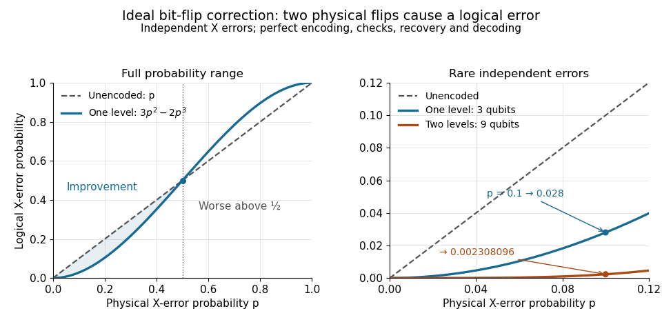
This calculation describes ideal correction of stored information with the specified quantum bit-flip channel. Repeated correction in time additionally requires a fresh specified noise model for each interval; imperfect quantum gates, faulty measurements and correlated errors change the calculation. The timed bit flip during repetition-code syndrome extraction and exact encoded-state failure with a faulty parity check show concretely why this storage calculation alone is not a fault-tolerance result.
Three-qubit bit-flip syndrome table 2026-10-14
Measure the commuting stabilizer generators and in that order. Use error syndrome bit for eigenvalue and bit for eigenvalue . For the Pauli X gate on physical qubit , every row holds for arbitrary normalized . This ordered parity-check convention follows [ref]
https://www.preskill.caltech.edu/ph229/notes/chap7.pdf. Preskill, §7.1
:| Error | State before recovery | eigenvalues | Error syndrome | Recovery |
|---|---|---|---|---|
Each pair of computational basis words within a row has the same two parities. Consequently the projective measurement reveals the row without distinguishing its two amplitudes. For example, becomes under . Both checks give with probability one, and applying restores both coefficients exactly, including the relative phase .
One implementation uses two quantum ancillas initialized to . Two controlled-NOT gates from data qubits 1 and 2 to the first quantum ancilla write their parity; two more from data qubits 2 and 3 to the second quantum ancilla write the other parity. Measuring only the quantum ancillas in the computational basis gives . Measuring the individual data qubits instead would reveal the encoded computational basis value and destroy the unknown quantum superposition. The existing coherent syndrome extraction for the three-qubit repetition code uses the alternative ordered checks , so its bit labels differ from this table.
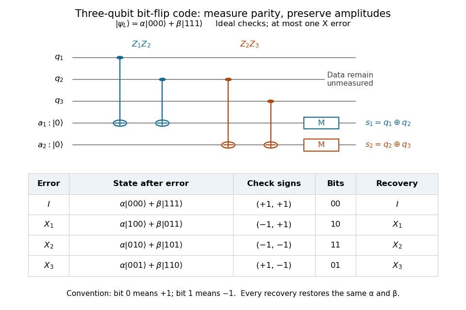


The recovery also handles coherent errors. Put . Their images of the code are mutually orthogonal, giving , the Knill--Laflamme condition for this family. For any linear combination , its component in sector is . Measuring that error syndrome has probability on the normalized erroneous state, and recovery returns . More generally one recovery quantum channel corrects every noise quantum channel whose Kraus operators belong to this span. The assumption concerns the whole jointly correctable family; it does not extend to the span of arbitrary single-site Pauli errors. [ref]
https://www.preskill.caltech.edu/ph229/notes/chap7.pdf. Preskill, §7.2: correction of an error span
.A fully computed coherent example is the unitary operator . At it givesThe error syndromes and occur with probabilities and , independently of . Doing nothing for and applying for restores the same logical qubit in both branches; the scalar in the second branch is an irrelevant global phase. This is an example of linearity of coherent quantum error correction, rather than an assumption that the original error was a classical random bit flip.
Limitations of bisection 2026-10-14
Several zeros of a function can lie in one initial root bracket: the bisection method seeks one, rather than enumerating them. For instance, the polynomial has opposite endpoint signs on , but its first midpoint evaluation returns only the polynomial root . The initial zero of a function need not be unique for the bisection error bound to apply to a retained zero of a function.
A zero of a function without a sign change cannot be located by the strict sign-change test alone. The polynomial touches zero at but is positive on either side. On both endpoint values are positive: although the closed interval contains a polynomial root, it fails the usual starting test for the bisection method. An endpoint or evaluated midpoint zero of a function can still be recognized directly.
Opposite signs certify a root bracket only with the required continuity. For , the values at and have opposite signs, but is undefined at the midpoint and has no zero of a function. Hence is invalid input for the bisection method; the intermediate value theorem does not apply across the gap.
Bisection stopping criterion 2026-10-14
For a requested absolute tolerance , stop when the retained root bracket has width at most , and report its midpoint. The bisection error bound then guarantees in exact arithmetic. Using the ceiling function and the base-two logarithm, the required number of halvings isThe zero allows stopping before any update when the initial root bracket is already sufficiently narrow. For the polynomial on with , . After nine halvings,Thus the reported midpoint meets the tolerance; its actual error from the square root is approximately . After eight halvings the bound is , so eight do not give this worst-case guarantee.
Cache the endpoint values. Each update of the bisection method needs just one new function evaluation, at the old midpoint. With no early zero of a function, updates therefore cost function evaluations, including the two initial endpoints. Returning the new midpoint requires no additional function evaluation; requesting its value would add one. The nine-update example needs eleven evaluations for the guarantee.
A small function value alone does not guarantee a small position error: rescaling changes those values without changing its zeros of a function. In a practical implementation, use an explicit width test and an iteration limit. With floating-point arithmetic, also stop if the computed midpoint equals either endpoint: the root bracket can no longer shrink, so repeating the update would loop forever. Report this precision limit separately if the requested tolerance remains unmet. Reliable sign evaluations are needed to preserve the root bracket; compare signs directly rather than multiplying endpoint values, which can suffer overflow or underflow in floating-point arithmetic.
For a rounded midpoint still inside a valid root bracket, the geometric error bound is ; it need not equal because of roundoff error. A rigorous computed enclosure also needs conservative arithmetic for that bound and reliable endpoint signs. The exact-arithmetic bisection error bound should not be claimed unchanged after precision prevents further halving.
For practical tolerance conventions, SciPy's
bisect combines absolute and relative tolerances through , and provides a maximum iteration count and convergence status. These differ from the purely absolute width test above.[ref]https://docs.scipy.org/doc/scipy/reference/generated/scipy.optimize.bisect.html. SciPy, scipy.optimize.bisect documentation
Bisection error bound Created 2026-10-14 Updated 2026-10-31
In exact arithmetic, after completed halvings the retained root bracket has width and midpoint , whereThe absolute value bound holds for every zero of a function in the current root bracket, including the one approached by continued bisection method updates. A zero of a function discarded with an earlier half need not satisfy later bounds. Before update , the evaluated candidate is , whose corresponding guarantee is . After update , the new midpoint has the smaller guarantee , even without evaluating .
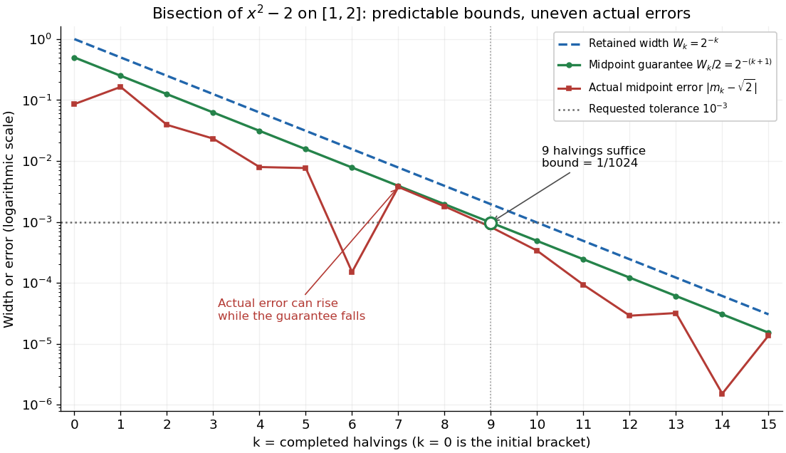
Bisection widths, midpoint error bounds, and actual square-root errors after zero to fifteen halvings
. Details. 
The guaranteed error halves at every step; the actual absolute value error need not decrease at every step or have successive ratio . In the square root example it increases from to , while both errors remain below their guarantees. An exact midpoint zero of a function instead gives zero error and immediate termination. For this example is an irrational number, so no finite exact halving can produce it as a midpoint.
For a brief proof outline, each retained half has half the previous width and contains a zero of a function by the intermediate value theorem. Every point in the retained root bracket is at most half its width from its midpoint. If the process does not stop at a zero of a function, the nested interval theorem gives one common point as the widths tend to zero; continuity and the opposite endpoint signs force its function value to be zero. Uniqueness in the initial root bracket is unnecessary.
There are unlisted articles, also show them or only show them.