
Beta sampling by uniform order statistics Created 2026-10-14 Updated 2026-11-05
For positive integers , the th order statistic from independent uniform distributions on has Beta distribution . Selecting the observations below and above a value gives its probability density function proportional to , with normalizing factor .
Moment matching for a beta prior Created 2026-10-14 Updated 2026-10-25
Moment matching for a beta prior turns a desired mean and variance for an unknown probability into the parameters of a beta distribution prior. Choose andSolving the beta distribution mean and variance identities givesThe strict upper bound on the variance makes , so both parameters are positive. Substitution gives mean and variance exactly. A smaller specified variance at fixed mean produces a more concentrated prior distribution.
For example, a desired prior mean and variance give , hence the beta distribution prior . With the same mean and variance , the calculation instead gives and the broader beta distribution prior . Both appear in the concentration diagram above.
The excluded boundary cases have clear meanings. Zero variance would require with certainty, not a beta distribution with finite positive parameters. At the other boundary, any random variable satisfies , hence variance at most ; equality requires to take only the endpoint values zero and one. This is a Bernoulli distribution, not a beta distribution. Thus cannot be matched by positive finite parameters, and or is also excluded.
After observing Bernoulli trials, the Beta-binomial conjugacy makes the posterior mean a weighted average of the prior mean and observed binomial proportion :This formula gives a precise interpretation as the prior's weight relative to the sample size in this posterior mean. It does not require fictitious observed counts: the beta distribution parameters can be any positive real numbers. For the eight-head, two-tail example above, and , so the posterior mean is .
// Target: statistical-inference.bigb
Sign criterion for best L1 approximation 2026-10-14
For real functions, let and put . If for every , then is a best approximation in a normed space using the norm. The proof is the pointwise inequality , followed by integration. This is a sufficient criterion even if the residual vanishes on a positive-measure set; a general necessary criterion may choose any subgradient in on that zero set.
For and , existence follows from finite-dimensional compactness and uniqueness from strictly convex normed space geometry. Translation by and negative translation by preserve the target and the error norm. Uniqueness forces the minimizing trigonometric polynomial to be invariant under the first operation and the negative of itself under the second. Invariance removes every nonzero frequency below ; negative invariance removes the remaining constant.
Put in the Bessel density modes of a polytropic expanding universe equation. It becomes . Substituting gives . Since , the fractional pressure correction is small when . For , this is the order-of-magnitude condition . It describes approach to the dust-like growing branch, not an exact universal time at which every initial perturbation starts increasing. The instantaneous Jeans instability balance instead compares with .
Perron tree 2026-10-14
A Perron tree is a finite triangular splitting-and-sliding arrangement retaining a prescribed angular range while overlapping its pieces strongly. The compression parameter and the number of generations can make union area an arbitrarily small fraction of total piece area. Suitable longitudinal extensions separate the pieces into disjoint rectangles. This stronger finite geometry is used by the ball-multiplier counterexample; a compact measure-zero Besicovitch set alone does not assert that arbitrary segment translates are disjoint.
Choose a compact with full horizontal projection and zero-length projections for . Then the displayed set is compact, has zero area by the Fubini theorem, and contains a segment of every slope in . Such parameter sets exist by the Baire category theorem in the Hausdorff metric: fine parallel segments approximate any parameter set while making a fixed band of projections uniformly small. Finite grids and a countable intersection make every required projection null. Four rotated copies supply every planar direction.
Typical-set indexing example 2026-10-14
The typical sequence theorem turns a probability concentration into a coding construction. Assign one binary number index to each weakly typical sequence, plus a reserved index for every word outside the set. The decoder recovers every typical word exactly; the reserved index has one predetermined output. The block code usesbits and has reconstruction-error probability at most .
For this example and , needs 34 bits but permits error up to about . At , 570 bits suffice and the error bound is about . These are existence calculations for an explicitly enumerated collection, rather than claims about an efficient practical encoder. The reduction comes from protecting the whole high-probability collection, rather than just its single most likely member.
Typical-set concentration for a biased coin 2026-10-14
The count has binomial distribution with mean and variance . The information content per symbol is an affine function of , so its variance isChebyshev's inequality therefore gives the finite-sample lower boundThe bound is often loose, but it proves that every fixed positive tolerance eventually captures nearly all the probability. Direct summation of the binomial distribution's probability masses gives . A finite sample does not need to have a nearly full typical set: the 40-symbol example above captures only about .
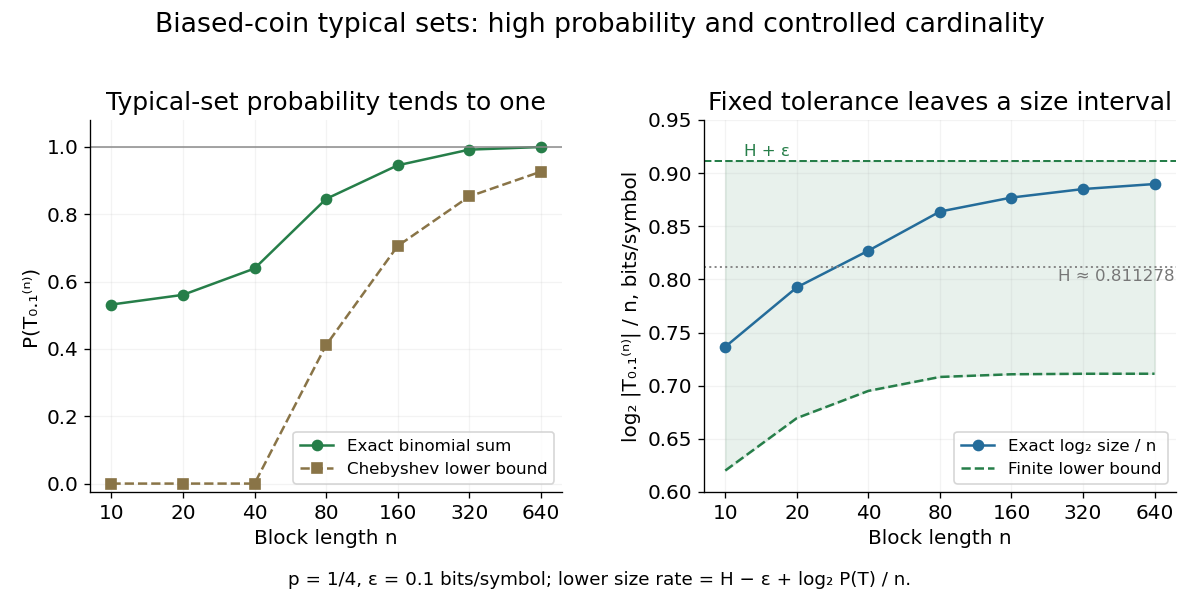
Longer biased-coin messages concentrate in typical sets with controlled size
. The left plot compares exact typical set probabilities with the lower bound from Chebyshev's inequality. The right shows and its finite-sample bounds. The tolerance stays fixed; the curve is not asserted to converge to exactly . All points are exact finite-model calculations. Details.
For , and , put while . Then . If , decreases to zero at the displayed finite time. The positive branch joins the zero solution with zero first derivative, giving a nonnegative forward solution. The equilibrium at zero is one-sided stable even though the vector field is not locally Lipschitz continuous there; the positive equilibrium is unstable.
Consider the original analytic initial value problemHere and are dimensionless variables in a stipulated mathematical model. The trajectories below are exact solutions of a differential equation, with no measured data or empirical parameter fit. For , the Bernoulli power substitution givesThe integrating factor is . Direct differentiation gives , independently checking the transformation. The linear exists for every real , while the nonlinear solution of a differential equation uses only the interval containing where :For , , so its absolute value decreases toward zero. The lost zero solution of a differential equation is recovered by substitution into the original equation. Since is locally Lipschitz in everywhere, the Picard-Lindelöf theorem ensures uniqueness through every finite point, including . Thus a nonzero trajectory never meets or crosses zero at a finite .
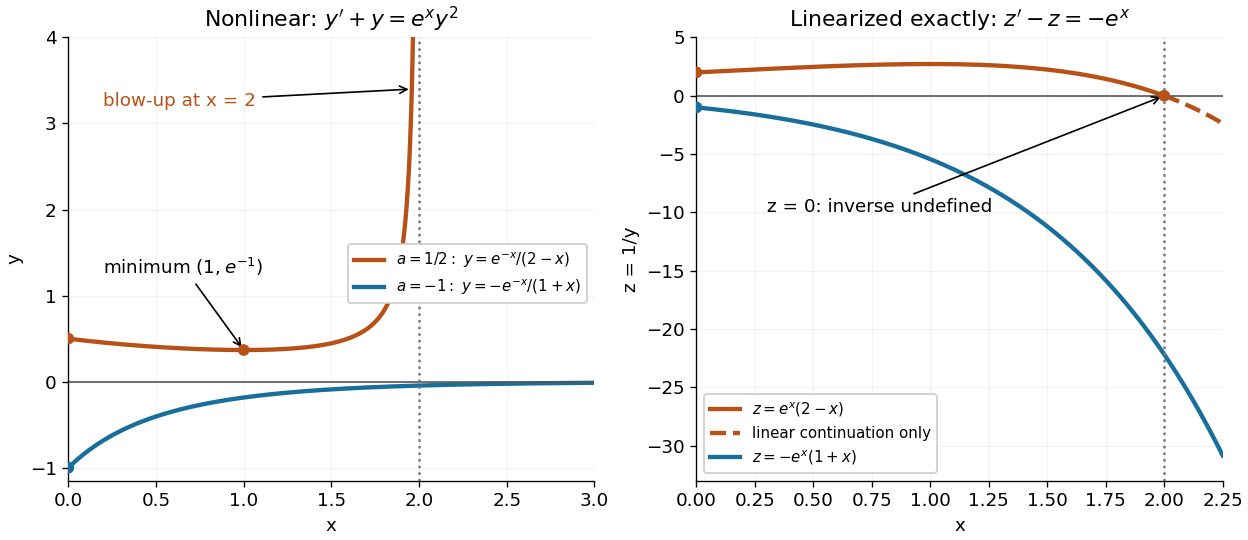
Two Bernoulli trajectories and their exact linearized coordinates
. The initial conditions are in orange and in blue. Left: the positive trajectory reaches finite-time blowup at , while the negative trajectory approaches zero. The vertical axis clips the positive curve at ; this is a display limit. Right: the corresponding trajectories satisfy . The dashed orange continuation past solves the first-order linear differential equation but cannot extend the original positive initial value problem across blowup. Details.
For , the exact solution of a differential equation is on . It first decreases, reaches a local minimum , then increases without bound. At the endpoint,The finite-time blowup comes from a simple zero of at , where , rather than from a singular coefficient in the first-order linear differential equation. The same algebraic expression for is negative on , but that is a separate solution of a differential equation on a disjoint interval; infinity supplies no finite joining value. For , on , giving a distinct decaying branch whose finite blowup is instead in the past.
The direction field also explains the positive turning point. Its nullclines are and , becauseAbove the positive nullcline, ; between it and zero, ; below zero, . The moving nullcline is not a solution of a differential equation: its derivative is , whereas the prescribed slope there is zero. The trajectory crosses it at , exactly its local minimum.
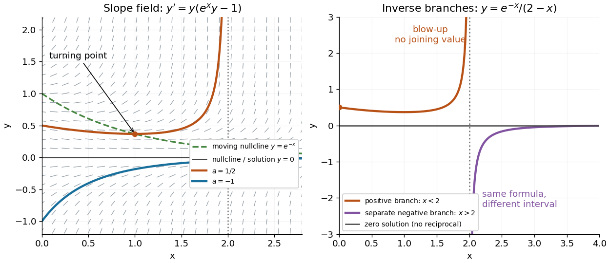
The Bernoulli direction field and the disconnected inverse branches at blowup
. Left: the direction field, its two nullclines, and the exact and trajectories. Right: has a positive branch on and a negative branch on ; the excluded point separates them. The zero solution of a differential equation belongs to the original equation but has no finite reciprocal coordinate. The branches continue beyond the plotted vertical limits. Details.
Bernoulli power substitution Created 2026-10-14 Updated 2026-10-25
For arbitrary real , work first on an interval where . Define exponentiation by , using the real logarithm. The change of variable is differentiable and invertible there, and the chain rule givesMultiplying the Bernoulli differential equation by yields the first-order linear differential equationThis is an exact transformation of nonzero solutions of a differential equation on the chosen branch; it is valid far from any reference state and does not discard higher powers as a local linearization would.
Given the initial condition , the integrating factor and transformed solution of a differential equation areThe product rule verifies . Recover only on the connected component of containing , inside the original coefficient interval. The first-order linear differential equation can have a longer existence interval than this inverse transformation allows.[ref]
1.4 Linear equations and the integrating factor. Notes on Diffy Qs, §1.4 Linear equations and the integrating factor: product derivative, formula (1.4), and Remark 1.4.1 on existence throughout a coefficient-continuity interval
Negative values need a separately justified real branch. For integer , the required powers are real and differentiable for too, but the inverse must retain the sign selected by the initial condition. For , represents either or ; both square roots are taken of positive . For , retains the sign directly. For a general noninteger exponent, use the positive branch unless a specific differentiable real negative branch has been established. Never evaluate a real fractional power of a negative value merely because the linear formula has become negative.
Division by excludes . When and the original real power is defined at zero, is an additional solution of a differential equation and must be checked in the original equation. When , the equation as written is undefined at zero. On a positive branch the right-hand side is locally Lipschitz in , so the Picard-Lindelöf theorem gives local uniqueness. At zero, the same hypothesis needs a fresh check: it holds for the polynomial example, whereas for a nonzero power coefficient prevents local Lipschitz continuity there. If , the inverse sends for , but sends for . The latter endpoint can lead to finite-time extinction in a sublinear Bernoulli equation, where the original equation determines how to join to zero.
Suppose a connection polynomial of degree at most , with recurrence span gives zero recurrence discrepancies through index but a nonzero discrepancy at . If a polynomial of span successfully explains the prefix through and , evaluate the coefficient at in the convolution . Applying first makes it zero. Applying first leaves its nonzero discrepancy at , because the earlier discrepancies vanish and has constant coefficient one. This contradiction gives the displayed lower bound. It is the minimality step used by the Berlekamp-Massey algorithm; the algorithm cancels the new discrepancy with a shifted earlier failed polynomial.
Vortex-pair renormalization flow Created 2026-10-14 Updated 2026-10-18
In the dilute-vortex description of the two-dimensional XY model, is dimensionless stiffness and is phase vortex fugacity. A phase vortex has logarithmic energy , while its placement entropy is . Small phase vortex pairs screen the logarithmic interaction, lowering the stiffness. Near , the rescaled variables , obey , to leading order. The invariant leads to an essential correlation-length singularity , not a finite power-law exponent.
Here increases toward larger observation distances, and the vortex fugacity is a dimensionless weight per unit core, conventionally initialized as with the microscopic measure fixed. Numerical coefficients depend on this normalization. In the displayed convention, differentiating using the original flow givesOnly replacing the prefactor by one near gives the scaled leading model. Its first integral follows directly:Thus this first integral belongs to the stated scaled model, not exactly to the original equations. For , the critical separatrix is . The bound side has and flows to , ; the unbinding side ultimately runs to large vortex fugacity, where the dilute approximation ceases to be quantitative.
To derive the unusual correlation length scaling without fitting an exponent, write the invariant on a nearby unbinding trajectory as . Then and the time to cross fixed small limits to is . If a physical one-parameter path crosses the separatrix transversely, its is proportional to the positive reduced temperature. Since distance grows as , this gives , with a nonuniversal . This is the dimensionless-temperature form of the singularity above.
For odd , multiplication by two permutes the residues modulo . Its orbit through is the binary cyclotomic coset modulo an odd integer. If has order in a finite field whose field characteristic is two, the Frobenius automorphism sends to . Hence the minimal polynomial of an algebraic element over is . Its coefficients are fixed by Frobenius and lie in , and its degree is the orbit size. Thus a binary cyclic code containing one defining zero of a cyclic code must contain the full orbit as zeros.
Designed distance 2026-10-14
The designed distance of a BCH code is the value specified by requiring consecutive defining zeros of a cyclic code. The BCH bound guarantees minimum Hamming distance at least , but the actual minimum Hamming distance can be larger. To prove equality, one can exhibit a nonzero codeword of Hamming weight exactly .
For a proper prior distribution independent of coalescent times , let with and . Observing under an infinite sites mutation model gives posterior density , where is the prior predictive probability of . Multiplication by the conditional Poisson mass and normalization is an application of Bayes' theorem.
// Target: statistical-inference.bigb
Posterior rank distribution 2026-10-14
For continuously distributed uncertain quantities, define rank one to be the largest. A joint posterior distribution induces a discrete distribution on each quantity's rank. Estimate it by ranking the whole vector in each joint draw and averaging rank indicators; the probability of rank one is the probability of being largest. Ranking posterior means does not recover this uncertainty. The joint draws must preserve any posterior dependence, and tie conventions must be specified for models with atoms.
Discrete uniform endpoint posterior 2026-10-14
For one uniformly sampled integer , the likelihood function for the unknown endpoint is . A flat improper prior on positive integers gives an improper posterior distribution, since the harmonic series diverges. A reciprocal prior instead gives a proper posterior proportional to for , with approximate survival probability and finite quantiles, but infinite posterior mean. A uniform prior cut off at gives posterior mean , demonstrating sensitivity to that arbitrary cutoff.
Bounded uniform-location posterior 2026-10-14
For independent observations uniform on and a uniform prior on , the likelihood is constant wherever all data-compatible intervals overlap. The posterior is therefore uniform on the displayed intersection, provided it has positive length. Both squared-error and absolute-error Bayes estimates are its midpoint. An empty or zero-length interval has zero marginal likelihood and cannot be normalized into this ordinary posterior density.
There are unlisted articles, also show them or only show them.