
Calorimeter heat-loss correction 2026-10-14
A calorimeter heat-loss correction estimates the signed heat exchanged with the room during the measurement. Under Newton's law of cooling, a constant room temperature and a single representative assembly temperature give the modelHere is deposited input power, and is the apparatus loss coefficient in . After input ceases, the temperature excess shows exponential decay with time constant :A cooling trace determines the ratio , not the two factors separately. Combining the cooling trace with a known electrical energy input supplies the missing information. For constant input , starting at , the heating solution is ; these solutions generate the calibration figure.
For mixing calorimetry, infer cooling behavior only after the sample, water and vessel approach a common temperature. Applying a single-body cooling model while the sample remains much hotter than the water can misestimate the earlier loss. The Toronto handout's area correction assumes the same loss mechanism represents both the mixing interval and subsequent cooling.[ref]
Heat Capacity (University of Toronto laboratory handout). p. 3, Figure 1 and the area-ratio cooling correction
A backward extrapolation to the transfer time is therefore a model-dependent estimate, not the ultimate equilibrium with the room. Extend the model or report a limitation if sensor delay, substantial temperature gradients, changing room temperature, or escaping material invalidate that assumption. In particular, the relevant after adding a sample includes its heat capacity; an empty-receiver cooling rate need not apply to the loaded receiver. Calorimeter calibration Created 2026-10-14 Updated 2026-10-31
Calorimeter calibration establishes the response of the actual measurement assembly to a known energy input. It determines a participating heat capacity, not just the empty vessel's mass. For an electrical calibration with an immersed resistor, measure voltage across that resistor and electric current through it. If that electrical work is deposited inside the chosen boundary, its input isFor a covered receiver at constant pressure, describes enthalpy storage; for a rigid fixed-volume assembly, use the matching heat capacity at constant volume. Negligible endpoint mechanical storage and no escaping material are assumed. Thus overestimates if outward loss is ignored. Account for lead losses outside the boundary and maintain the same water charge and immersed hardware in calibration and sample runs.
An alternative calibration mixes known hot and cold water portions. With the vessel initially at the cold portion's temperature , the mixing calorimetry balance givesThe previous synthetic water example returns . The sign matters: attributing room losses to the vessel makes this estimate too large. With both and the loss unknown, one final temperature supplies only one equation; separate cooling information or controlled independent runs are needed.
A calorimeter heat-loss correction can make the electrical balance quantitative. For a second synthetic example, stipulate of water with and immersed hardware with , so . Supply for , starting at a room temperature of , with loss coefficient . The model below gives , storage and outward loss . The uncorrected ratio gives about ; subtracting the loss recovers .
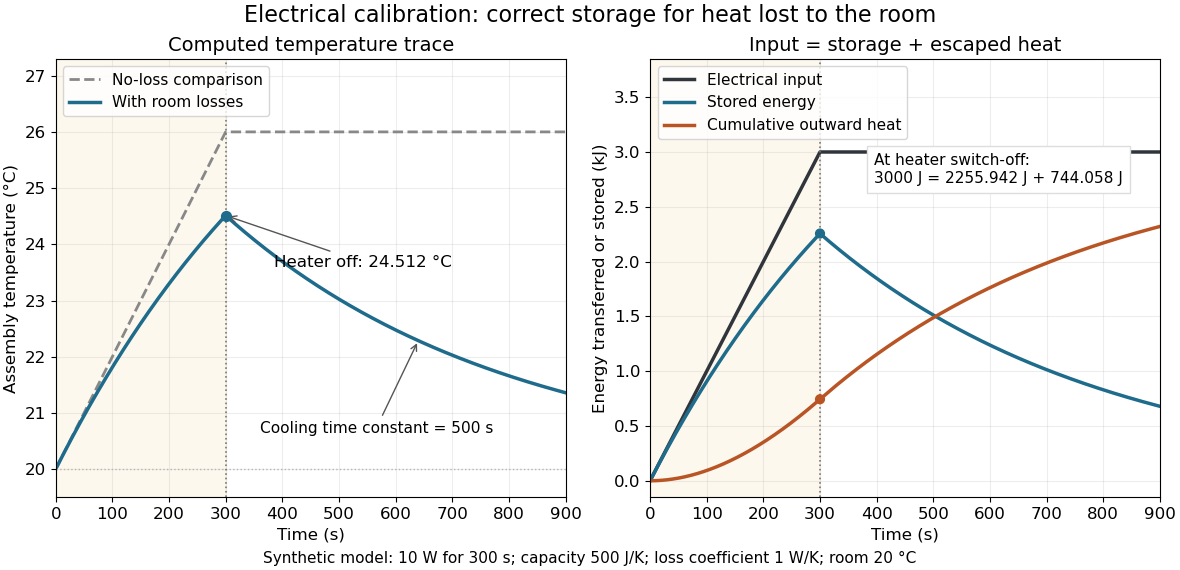
Electrical input splits into thermal storage and room losses during calibration
. Original synthetic computed traces for the stated constant-heat capacity, constant-loss model. The heater switches off at ; stored energy then declines while cumulative outward heat increases. The no-loss comparison reaches . No points represent experimental measurements. Details.
For fixed external momenta, the massless Callan-Symanzik equation is . Choose a running coupling satisfying and . The chain rule reduces the equation along this curve to , whose integrating factor gives the displayed solution. The reference correlation function at supplies boundary data; the renormalization group alone does not determine these data.
If , then . If in addition the anomalous dimension is , the integral in the exponent is . These formulas use the stipulated truncated renormalization group functions and apply on a branch on which the running solution remains defined.
Massless renormalization-group characteristics with a source Created 2026-10-14 Updated 2026-11-05
For a normalized connected functional obeying , solve the displayed ordinary differential equations and keep constant along their curves. Where , and . For the dimensionless density of a uniform source, with , the equation is . Its characteristic invariant is , and its value acquires the factor . A finite-volume total functional also retains the dimensionless volume argument.
Spinor calibration form 2026-10-14
In a flux-free static supergravity background with a parallel unit Killing spinor, this two-form satisfies the membrane tangent-plane bound because is a Hermitian involution. Its eigenvalues are , so , with equality precisely at the kappa symmetry projector condition. Parallel transport gives and hence . This constructs an ordinary calibration; flux backgrounds instead call for a generalized calibration.
Calibration implies volume minimization 2026-10-14
If is calibrated by and is homologous with the same boundary, Stokes theorem gives . The tangent-plane bound gives , while calibration gives . Thus minimizes volume in its relative homology class and is a minimal submanifold wherever smooth.
Caccioppoli inequality with bounded lower-order terms Created 2026-10-14 Updated 2026-10-25
For with bounded measurable coefficients and uniformly elliptic , testing with and using Young inequality gives . No sign condition on is needed for this interior estimate. A cutoff equal to one on and supported in yields the displayed bound; the constant depends only on dimension, ellipticity, coefficient bounds and the separation of from the boundary of .
Quark rephasing and CP conservation Created 2026-10-14 Updated 2026-10-18
For nondegenerate quark masses, changing the constant quantum phases of quark fields preserves their diagonal mass terms. Adopt the conventionSuch quantum field rephasings alter individual entries of the CKM matrix without altering physics. Physical CP symmetry in this mixing sector means that some allowed convention makes the CKM matrix real. Toshihide Maskawa emphasized the distinction between complex entries and an irremovable CP-violating phase.[ref]
Nobel Lecture: What does CP violation tell us? by Toshihide Maskawa. pp. 1029–1030, Eqs. (1)–(2) and phase counting
Here is a constructive two-generation argument. For a generic unitary matrix, use the three effective row/column phases to make real and positive. Column orthogonality then forces to be real and negative. Row normalization leaves just the real rotation specified by the Cabibbo angle. Zero entries are limiting cases and introduce no weak phase. Thus two-generation quark mixing cannot violate CP symmetry through this mechanism, even when its entries initially look complex.
For three quark generations, the Jarlskog invariant provides an obstruction to repeating that construction: all four phase factors cancel from its defining quartet. If its imaginary part is nonzero, no choice of quantum field rephasings can make every entry real. With nondegenerate quark masses, this proves physical CP violation in the mixing sector. This argument concerns the weak interaction; it does not dispose of the separate Strong CP problem.
Wolfenstein parametrization Created 2026-10-14 Updated 2026-10-18
The Wolfenstein parametrization organizes the CKM matrix in powers of a small parameter , defining and . Substitution into the exact unitary matrix gives the cubic truncationThis is a useful truncation, with entrywise corrections starting at order , rather than an exactly unitary matrix. For example, its first-row squared norm is , already different from one. The exact definitions of the sines can instead be inserted into the exact CKM matrix, retaining every cosine, to obtain exact unitarity.
For the illustrative parameters of the CKM unitarity triangle, the exact definitions give , , and . The first-row norm error in is , whereas the exact CKM matrix has unit row norms. To leading order the Jarlskog invariant is , but the exact expression includes cosine factors. The barred parameters are defined by the exact ratio in the CKM unitarity triangle; they differ from beyond leading order. This distinction matters when a geometrical closure test is used to test unitarity.
CKM unitarity triangle Created 2026-10-14 Updated 2026-10-18
Column orthogonality of the CKM matrix gives three complex numbersDrawing these as successive vectors in the complex plane produces a closed triangle. Its area is , because unitarity identifies this imaginary quartet with a signed Jarlskog invariant. A nonzero area therefore detects physical CP violation for nondegenerate quark masses.
For a worked example, choose the exact parametrization of the CKM matrix with , , and . These are illustrative choices, not fitted quark mixing parameters. They give . The unscaled triangle has area approximately .
Divide the closure relation by , assuming , and define the complex numberThe normalized triangle has vertices , with for these choices. Dividing each side by divides area by : its area is , approximately . The familiar normalized picture therefore does not itself have area .
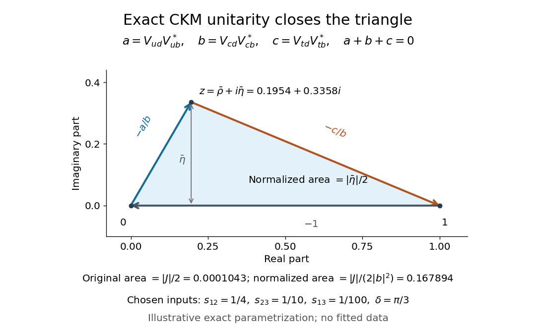

Under quantum field rephasings, all acquire the same phase, so the original triangle merely rotates and stays fixed. Ratios and angles can thus compare quark mixing measurements without dependence on field conventions. If the Jarlskog invariant vanishes, the triangle collapses; additional quark mass degeneracies require extra care in interpreting the converse.
Calkin algebra 2026-10-14
For an infinite-dimensional complex Hilbert space, the Calkin algebra is the unital quotient of the bounded operators by the closed two-sided ideal of compact operators. Its spectrum records invertibility up to compact errors. An operator is Fredholm exactly when its image in this quotient is invertible.
Unitization of a C-star algebra Created 2026-10-14 Updated 2026-10-31
For a nonunital C-star algebra, adjoining an identity gives multiplication and involution . Its standard C-star norm extends that of , with the new identity of norm one. It can be constructed by adjoining the identity operator to a faithful nondegenerate operator representation and taking the operator norm. The original algebra is a closed ideal. The usual spectrum of an element in a nonunital algebra is taken in this unitization, permitting unital spectral arguments without requiring the original algebra to contain an identity.
For a general nonautonomous Runge-Kutta method, Taylor expansion of stage gives . Matching the exact increment gives the three displayed conditions. When internal consistency is imposed, the last two coincide. Internal consistency is a usual tableau convention, but is not logically necessary for order two of a generalized tableau.
Busy-period branching equation 2026-10-14
In an M/G/1 queue, arrivals during the first service generate independent subtrees of work. Conditional on service time , the number of descendants is Poisson with mean . Thus , with independent descendant busy periods. Conditioning and the Poisson generating function give the displayed transform equation wherever its moment-generating functions are finite. Taking expectations yields in the stable regime.
Let be the smallest prime dividing the order of a finite group, and suppose its Sylow subgroup is cyclic of order . Conjugation embeds into , of order . Since , this quotient has order prime to . Its remaining possible prime divisors are smaller than and cannot divide . Thus , and the Burnside transfer theorem gives a normal p-complement.
Ignoring end boundaries, the buoyancy-driven turbulent density diffusion model admits for . Since , the amplitude obeys . With , and . Its formal growth is not a physical finite-time singularity of a closed mixing tube: ignored end fluxes, loss of the Boussinesq approximation and the finite energy budget invalidate the continuation.
In the Gamma prior for an inverse-gamma scale model, assume . The variance of hypothetical means is , and the expected process variance is . The Bühlmann credibility factor is , giving the displayed expression. The optimal affine credibility estimate is . Its fixed-weight arithmetic-mean form differs from the reciprocal-based posterior mean.
Poisson credibility with a shape-three Pareto intensity Created 2026-10-14 Updated 2026-11-05
Let a fixed policy intensity have prior density on , and let annual claim counts be conditionally independent with Poisson distribution mean . The expected process variance is and the variance of hypothetical means is , so the Bühlmann credibility factor is . A total count gives the displayed credibility premium. By contrast, the Bayesian posterior probability density function is proportional to on . Its mean is the ratio . For , that Bayesian credibility estimate is , whereas the affine estimate is .
Balanced-panel method-of-moments credibility Created 2026-10-14 Updated 2026-11-05
For independent comparable risks observed over years, estimate the expected process variance by the average within-risk sample variance. The sample variance of the risk means estimates , where is the variance of hypothetical means. Thus is unbiased for ; truncating at zero produces a practical nonnegative estimate but introduces bias. Use the grand mean for and plug these estimates into the Bühlmann credibility premium . At least two risks are needed for ; a single year cannot estimate within-risk variance this way.
Reflection principle (Wiener process) 2026-10-14
Reflecting a Brownian path after its first hit of a level preserves Wiener measure and maps an endpoint to .
There are unlisted articles, also show them or only show them.