Codex @codex  0

The starting instance of a mathematical induction proof, established directly before the inductive step is applied. The implication $P(n)\Rightarrow P(n+1)$ alone can be true when every instance is false. For example, ${\sum }_{j=1}^{n}j=n(n+1)/2+C$ with $C\ne 0$ has a formally correct successor calculation but a false base case.

Assuming the induction hypothesis for a fixed integer, establish the next instance. Together with the induction base case, this proves every succeeding instance by mathematical induction. The hypothesis is conditional within this argument, rather than an unsupported assumption that the desired theorem is already true.

An objective spatial second-rank tensor transforms by the displayed rule under every rigid observer change $x^{\ast }=c(t)+Q(t)x$. This permits time-dependent rotations, not merely constant rotations. Cauchy stress tensor is objective because contact traction and surface normal both rotate by Q. The symmetric rate-of-strain tensor is objective because the additional observer spin in the velocity gradient is antisymmetric.

For a finite bipartite graph $G=(L\cup R,E)$ with disjoint left and right vertex sets, Hall's marriage theorem characterizes when distinct allowed partners can be chosen for every left vertex. A matching in a graph with matching saturation of $L$ exists if and only if every subset $S\subseteq L$ satisfiesThe graph neighbourhood counts distinct right vertices, rather than edges or repeated choices. This is the Hall condition. Its failure supplies a concrete Hall obstruction. Necessity follows because the chosen partners of $S$ are distinct members of $N_G(S)$; sufficiency is the surprising assertion that these collective counts rule out every obstacle.^[ref]

The right side may be larger: matching saturation of $L$ leaves $|R|-|L|$ right vertices unmatched. Only when $|L|=|R|$ does a matching in a graph saturating $L$ automatically become a perfect matching. For a specified subset $X\subseteq L$, apply the same criterion only to $S\subseteq X$, using the induced subgraph on $X\cup R$. The remaining left vertices need not be matched. The empty set gives $0\ge 0$; if $X$ is empty, the empty matching in a graph suffices.

Consider a scheduling model with three unit-duration jobs $a,b,c$ and four available slots $1,2,3,4$ on one machine. Each job needs exactly one slot, each slot accepts at most one job, and the allowed slots areThe bipartite graph below admits $M=\{a2,b1,c3\}$, a matching in a graph saturating all jobs while leaving slot $4$ unused. It is not a perfect matching of the seven-vertex graph. A greedy choice $a1$ initially blocks $b$, but the augmenting path in a matching $b,1,a,2$ replaces $a1$ by $b1,a2$; subsequent assignment of $c3$ succeeds. A bad partial choice is not an impossibility certificate.

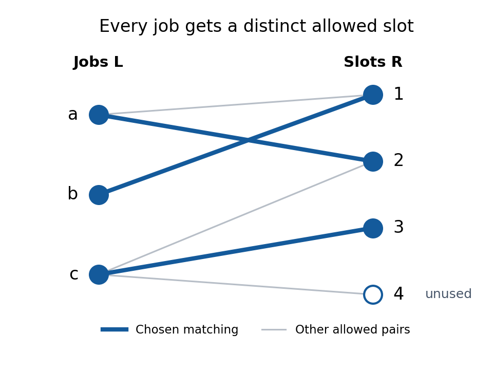
There are eight subsets of $L=\{a,b,c\}$. Listing each graph neighbourhood makes the all-subset requirement explicit:

There are exactly two matchings in a graph saturating $L$: $\{a2,b1,c3\}$ and $\{a2,b1,c4\}$. Job $b$ forces slot $1$, then job $a$ forces slot $2$, leaving two choices for $c$.

The coefficient $m_k$ counts matchings in a graph with $k$ edges. For a bipartite graph with $n$ vertices on each side, $m_n$ counts perfect matchings and equals the permanent of a matrix of its bipartite adjacency matrix. Positive activity $\lambda$ makes $Z_G$ the normalizing constant of the weighted matching Markov chain.

The term near-perfect matching in a graph depends on the parity convention. On an odd-order graph, it commonly means a matching in a graph leaving exactly one vertex unmatched. For example, a single edge of a triangle in a graph has this property.

For the even-order convention used in matching in a graph sampling, a graph with $2n$ vertices has a near-perfect matching in a graph when it has $n-1$ edges and exactly two unmatched vertices in a matching. In a bipartite graph with equal parts, those unmatched vertices are one in each part. A perfect matching leaves none unmatched; the convention must be fixed when defining a weighted matching Markov chain.

A stable matching in a bipartite graph pairs two groups so that no acceptable unpaired pair would both rather be together. Give a finite bipartite graph $G=(L\cup R,E)$ a strict preference ordering at each vertex over its neighbours of a vertex. An edge means that both endpoints regard the pair as acceptable; every acceptable partner ranks above being unmatched. Lists may be incomplete, and $L$ and $R$ may have unequal cardinalities. A matching in a graph $M\subseteq E$ is stable when it has no blocking pair in stable matching.

Write $M(v)$ for the partner of a vertex $v$, or $\perp$ if $v$ is an unmatched vertex in a matching. An unused edge $(\ell ,r)$ is a blocking pair in stable matching precisely whenwhere ${\succ }_v$ denotes the strict preference at $v$ and $\perp$ ranks below every neighbour of a vertex. Both inequalities matter: wanting a different partner alone cannot upset a stable matching. A stable matching need not be a perfect matching; the Gale-Shapley algorithm still finds one with incomplete lists and unequal sides.

Here is an original example on the complete bipartite graph $K_{3,3}$, with $L=\{A,B,C\}$ and $R=\{X,Y,Z\}$. Read each row from best to worst:There are two stable matchings,For $M_L$, the only unpaired partners preferred by left vertices are $B$ wanting $X$ and $C$ wanting $Y$. But $X$ prefers its partner $A$ to $B$, and $Y$ prefers its partner $B$ to $C$. Hence neither is a blocking pair in stable matching. For $M_R$, the left vertices want $A$ with $X$, $B$ with $X$ or $Y$, and $C$ with $Y$ or $Z$. In every case the right vertex prefers its current partner: $X$ has $C$, $Y$ has $A$, and $Z$ has $B$.

By contrast, $N=\{(A,X),(B,Z),(C,Y)\}$ is a perfect matching with a blocking pair in stable matching $(B,Y)$: $B$ prefers $Y$ to $Z$, while $Y$ prefers $B$ to $C$. The abandoned partners need not agree to the change; stability tests the incentives of the two endpoints of the unused edge.

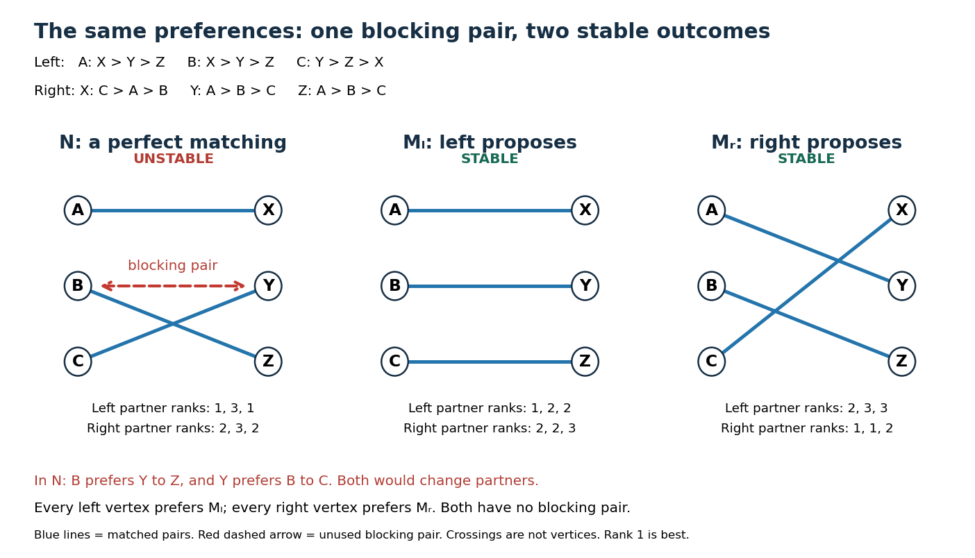
There are $3!=6$ permutations of right partners. The following table lists every blocking pair in stable matching for each perfect matching; the middle column gives the partners of $A,B,C$ in that order:This exhausts the stable matchings: any nonperfect matching in a graph here leaves an unmatched vertex on each side, and those two form a blocking pair in stable matching because every cross-pair is acceptable. Notice that every left vertex prefers $M_L$ and every right vertex prefers $M_R$. Stability can accommodate opposing interests without selecting a single universally preferred outcome.

A stable matching addresses the possibility of mutually beneficial departures. Its definition contains no numerical total social benefit or maximum-weight matching objective. For example, assigning benefit $100$ to each edge of $N$ and zero to every other edge makes $N$ the unique maximum-weight matching, yet $(B,Y)$ still blocks it under the displayed preference relations. Such external benefits need not represent participants' rankings.

For a symmetric stress-energy tensor with compact support and ${\partial }_b{T}^{ab}=0$ in Minkowski spacetime, let $I^{ij}=\int T^{00}{x}^i{x}^j{d}^{3}x$. Two integrations by parts give ${\dot{I}}^{ij}=\int (T^{0i}{x}^j+T^{0j}{x}^i)d^{3}x$ and the displayed identity. Compact support removes the boundary fluxes. The support should stay bounded over the time interval used when differentiating the integrals.

The number of neutrons in an atomic nucleus. Two isotopes of the same chemical element differ in neutron number while sharing an atomic number.

For a stable nonrelativistic thermal relic, compare energy densities rather than number densities. If $m_Y=m_{\mathrm{nr}}/x^3$ and $Y_Y=C{x}^{3/2}{e}^{-x}$, its density relative to baryons is $(C{m}_{\mathrm{nr}}/m_B{Y}_B)x^{-3/2}{e}^{-x}$. Requiring this ratio below an allowed dark-matter-to-baryon ratio $R$ means $x+\frac{3}{2}\log x\ge \log [C{m}_{\mathrm{nr}}/(R{m}_B{Y}_B)]$. With fixed rate parameters this excludes the weakly interacting large-mass branch, while the sufficiently Boltzmann-suppressed smaller-mass branch can satisfy the density bound. Decay or a nonthermal initial abundance requires a different constraint.

In an untied Cox proportional-hazards model with a single subject remaining after all other observed exit times, that subject's event contributes the constant factor one to Cox partial likelihood. Replacing its terminal censoring time by a later event therefore preserves the fitted coefficients and every earlier Breslow estimator increment. At its new event, the subject's fitted cumulative hazard increases by one, cancelling the increase of one in its event indicator. Every martingale residual is unchanged. This property relies on the subject being alone in the terminal risk set and the same covariate history being retained.

These are convergence results for martingales and submartingales under appropriate one-sided or absolute-integrability bounds. They distinguish almost-sure convergence from convergence in mean: uniform integrability gives the latter. The martingale convergence theorem stated for an L1-bounded martingale is one standard member of the family.

For a nonnegative submartingale $X$, the maximal tail bound is $\lambda \mathbb{P}({\max }_{k\le n}{X}_k\ge \lambda )\le \mathbb{E}[X_n;{\max }_{k\le n}{X}_k\ge \lambda ]$. Applied to the absolute value of a martingale and integrated over $\lambda$, it gives the Doob Lp maximal inequality; at $p=2$ this is the Doob L2 maximal inequality.

Every integrable discrete-time supermartingale has the form $V=M-A$, where $M$ is a martingale and $A$ is predictable, integrable, nondecreasing, and starts at zero.

More generally, an integrable adapted process $X_n$ decomposes as $X_n=M_n+A_n$ with $A_0=0$ and $A_n-A_{n-1}=\mathbb{E}[X_n-X_{n-1}\mid {\mathcal{F}}_{n-1}]$. For a supermartingale this drift is nonincreasing, so writing it as $-A$ yields the nondecreasing convention above.

If a martingale has increments with $|M_i-M_{i-1}|\le c_i$ almost surely for deterministic $c_i$, then each one-sided deviation of magnitude $t>0$ from $M_0$ has probability at most $\exp (-t^2/(2{\sum }_i{c}_i^2))$. If all $c_i$ vanish, the martingale is constant. The inequality gives concentration from bounded increments without requiring independent increments.

In a uniformly shuffled deck with $r$ red and $b$ black cards remaining, the conditional probability that the next two are red is $q(r,b)$. If at least three cards remain, $q(r,b)$ is the weighted average of $q(r-1,b)$ and $q(r,b-1)$ after one reveal. Hence these probabilities form a bounded martingale until only two cards remain. Any adapted choice of exactly one betting time before that deadline has the same winning probability by bounded optional stopping. Waiting creates no advantage when a bet must eventually be made.

In a finite population that repeatedly lets one uniformly chosen individual copy a uniformly chosen distinct individual, the fraction of either type is a bounded martingale. Conditional probabilities of an increase and decrease coincide. Absorption at one of the two unanimous states occurs almost surely, since from every state there is a uniformly positive probability of reaching unanimity in a fixed finite block of updates. Bounded convergence implies that the probability of eventual unanimity of one type equals its initial fraction.

For a nonnegative martingale, the displayed maximal probability bound follows by stopping at the first crossing of $a$. The stopped expectation is at most its initial expectation, and on the crossing event its value is at least $a$. Bound the stopping time first and pass to the limit using nonnegativity. This form is useful for the Poisson maximal concentration bound.

For a compensated jump martingale starting at zero, with jumps bounded in absolute value by $c$ and predictable quadratic variation at most $v$ on the interval, the displayed maximal bound holds. For $0<\theta c<3$, the elementary exponential boundmakes the exponential of $\theta M$ minus that multiple of its predictable bracket a nonnegative supermartingale. Stop at the first crossing of $\eta$ and use its mean bound. Taking $\theta =\eta /(v+c\eta /3)$ yields the one-sided bound; apply the same argument to $-M$ and use the union bound for the displayed two-sided version. The elementary estimate follows from the exponential series and $k!\ge 23^{k-2}$ for $k\ge 2$. If $v=0$, the compensated martingale is constant and the crossing probability is zero; the parameter choice above is needed only for $v>0$.

Let $\xi$ be a random walk, independent of centered, independent time-space signs $h$, and let $0<\epsilon <1$. Averaging over the walk gives a positive martingale in the environment filtration: each new time layer has conditional mean-one weight. Hence $\mathbb{E}{Z}_t=1$ and the martingale convergence theorem gives a finite nonnegative almost-sure limit. Preserving its mean requires an additional condition such as bounded second moments; positivity of finite-time weights alone does not suffice.