
Cell fate Created 2026-10-14 Updated 2026-10-20
Cell fate is the developmental outcome of a biological cell or its descendants in a specified setting. What it normally becomes and what it can become after an experimental intervention are different questions. The intestinal nucleus transfer experiment tests potential after cellular reprogramming, rather than directly tracing the normal cell fate of the donor.
Wee1 Created 2026-10-14 Updated 2026-10-14
Wee1 is a protein kinase that inhibits CDK1 by adding a phosphate group at an inhibitory site. Purified human Wee1 phosphorylated Cdc2 at Tyr15 in the reported in vitro assay, with no Thr14 modification detected. A catalytic-site mutation abolished both the measured protein kinase activity and the ability to inhibit division. This identifies a catalytic brake rather than merely a correlated protein amount.[ref]
Human Wee1 kinase inhibits cell division by phosphorylating p34cdc2 exclusively on Tyr15 by Clare McGowan and others. McGowan and Russell (1993), abstract: purified human Wee1, Tyr15 specificity, no detectable Thr14 phosphorylation, and Lys114 mutant control
Do not attribute all inhibitory CDK1 phosphorylation to Wee1: the Xenopus laevis Myt1 experiment separately identified activity toward both Thr14 and Tyr15. Nor does every phosphorylation inhibit its target: activating Thr161 modification in the studied Xenopus laevis Cdc2 has the opposite role. In cell-cycle activation feedback, suppression of Wee1 removes a brake on CDK1, reinforcing the transition without implying that the total amount of either protein instantly disappears.
Cdc25 Created 2026-10-14 Updated 2026-10-14
Cdc25 is a protein phosphatase: it removes inhibitory phosphate groups from CDK1, relieving inhibition of an appropriately prepared cyclin B–CDK1 assembly. Its reaction is removal, whereas Wee1 is a protein kinase adding inhibitory modification. Removing the inhibitory sites is different from removing the activating phosphorylation supplied by CAK.[ref]
Components of the Cell-Cycle Control System. Components of the Cell-Cycle Control System: inhibitory phosphorylation and Figure 17-18, Cdc25-mediated removal of inhibitory phosphates
Cdc25 action on CDK1 must also be distinguished from phosphorylation of Cdc25 itself. In cell-cycle activation feedback, CDK1-dependent regulation promotes Cdc25 activity, which can then activate additional inhibited CDK1. The complete regulatory path can involve intermediates. A histone H1 kinase assay of a mixture reports downstream protein kinase action; assigning its change to Cdc25 requires a perturbation or an independent protein phosphatase assay, rather than interpreting histone H1 labeling as phosphate removal.
Cyclin B Created 2026-10-14 Updated 2026-10-14
Cyclin B is a regulatory protein partner of CDK1. The protein kinase catalytic component is CDK1; bound cyclin B helps make that component competent to act. Changes in cyclin B synthesis and destruction regulate how much assembly can form, while CDK1 phosphorylation states determine whether bound assemblies are inhibited. This separates the supply of regulatory partners from release of an already assembled brake.[ref]
Components of the Cell-Cycle Control System. Components of the Cell-Cycle Control System: cyclically activated protein kinases, Figures 17-15–17-17, and “Cdk Activity Can Be Suppressed Both by Inhibitory Phosphorylation and by Inhibitory Proteins”
More cyclin B therefore need not give a proportional increase in CDK1 activity. Compare the matched-input cell-cycle hysteresis experiment, where different histories produced different activities, and the distinct measurements under CDK1 activity and protein abundance. Neither comparison makes cyclin B itself the catalytic protein kinase.
Cyclin-dependent kinase 1 Created 2026-10-14 Updated 2026-10-14
Cyclin-dependent kinase 1, abbreviated CDK1 and historically called Cdc2, is the catalytic protein kinase in the CDK1–cyclin B assembly. CDK1 transfers a phosphate group from ATP to a protein substrate; cyclin B supplies a regulatory binding partner. Binding and phosphorylation regulate catalytic competence, so detecting CDK1 protein alone does not establish activity. The distinction makes a durable catalytic component reusable as the cell cycle changes its regulatory inputs.[ref]
Components of the Cell-Cycle Control System. Molecular Biology of the Cell, 4th edition, Components of the Cell-Cycle Control System: “The Cell-Cycle Control System Is Based on Cyclically Activated Protein Kinases”, Figures 17-15–17-16
The cell-cycle activation feedback uses CDK1 activity as both an output and a regulatory input: activity promotes Cdc25 activation and suppresses Wee1, reinforcing release from inhibitory phosphorylation. The already described cell-cycle hysteresis experiment tests how that output depends on history at matched cyclin B input; the histone H1 kinase assay below explains what its output measures. A binding diagram alone cannot establish hysteresis.
Cell-cycle hysteresis experiment 2026-10-14
A 2003 study split a Xenopus laevis egg extract into portions with different histories. One received calcium to destroy endogenous cyclin B before receiving nondegradable cyclin B; the other received nondegradable cyclin B first, then calcium. The same sustained cyclin B dose was approached from low or high Cdc2 activity. A phosphorimager quantified histone H1 phosphorylation, sampling every – minutes until an apparent stationary response. At –, the dose maintained high activity but failed to induce it from the low state.[ref]
Controls tracked labeled endogenous cyclin B disappearance after calcium treatment and persistence of nondegradable cyclin B, addressing unequal remaining input. The comparison supports hysteresis under extract conditions; finite observations cannot establish indefinite persistence. It does not isolate each reinforcing path or establish thresholds in intact biological cells.[ref]
Building a cell cycle oscillator: hysteresis and bistability in the activation of Cdc2 by Joseph R. Pomerening and others. p. 3, control discussion; p. 4, Figure 3h; reported 60–90 minute approach to apparent steady state
Closed-channel cell-flux constraint Created 2026-10-14 Updated 2026-11-05
A genuinely closed steady channel with impermeable sidewalls and ends must have zero integrated axial cell flux through every section, not only zero fluid flux. In the bulk phototactic ansatz , , and , the axial flux is . Meanwhile the momentum equation, zero fluid flux and integration by parts give . Thus a nontrivial bulk profile is generally incompatible with exact closed-end cell conservation unless the prefactor vanishes. Additional axial concentration variation is needed; neglecting end regions does not itself remove this global constraint.
Prüfer sequence 2026-10-14
For , a Prüfer sequence is the encoding of a labelled tree on by a sequenceRepeated labels are allowed, and their order matters. To encode the tree, repeatedly remove its smallest-labelled leaf of a graph together with its incident edge, recording the label of its unique neighbour. Stop when two vertices remain; do not record their final edge. Removing a leaf of a graph leaves a tree, so the procedure makes exactly deletions. The choice of the smallest label makes the encoding deterministic. [ref]
https://users.math.msu.edu/users/magyarp/math481/. Peter Magyar, Math 481: Prüfer encoding with the smallest leaf
For a concrete example, take six vertices and the set of edgesInitially label the vertices of vertex degree one. Remove and record its neighbour . Now has become a leaf of a graph, so remove and record . Next remove and record again; then remove and record . The final edge joins and . Thus the Prüfer sequence isThe deletion order is : removing a leaf of a graph can make its neighbour a leaf of a graph, so the eligible labels change as the tree shrinks.
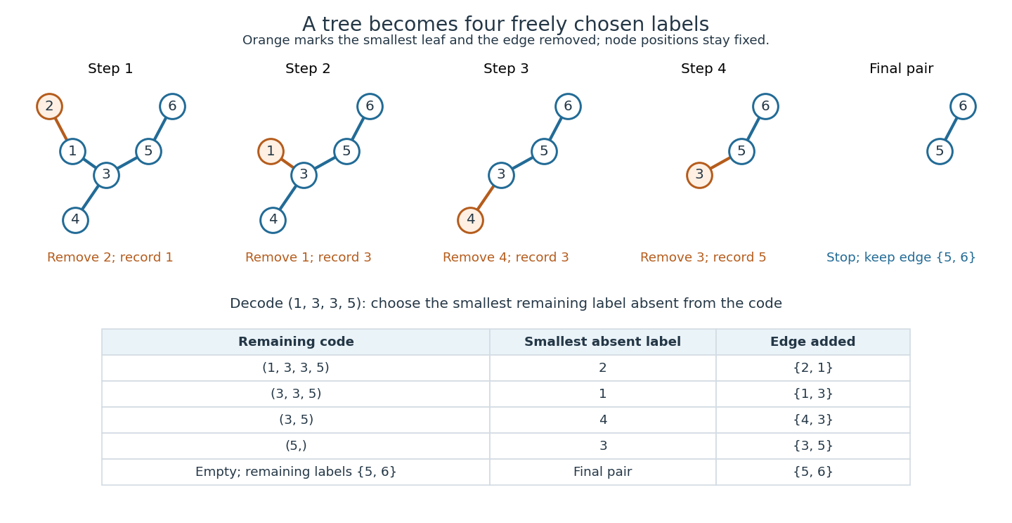

To decode, keep a set of remaining labels, initially , and the remaining sequence, initially . While the sequence is nonempty, let be the smallest label in absent from the entire remaining sequence. Add an edge between and its first entry, then remove from and delete that first entry. Finally join the two labels left in . For the example:
The decoder always has a choice: if the remaining sequence has length , then has labels, so at least two of them are absent. Its first entry is still in , and differs from the chosen absent label. Every removed vertex attaches to a vertex that survives longer; following these attachments eventually reaches the final pair. Consequently the decoded graph is connected, and its edges make it a tree. In this construction, each occurrence of contributes an incident edge, and gets one more edge at its final attachment. Thus a remaining label is absent from the remaining sequence exactly when it labels a leaf of a graph. Encoding and decoding choose the same smallest label at each step and undo each other. This bijection proves Cayley's formula and explains why every freely chosen sequence is valid. [ref]
https://www.cs.columbia.edu/~cs4203/files/GT-Lec4.pdf. Columbia University, Graph Theory Lecture 4: Prüfer degree identity, decoding algorithm, and bijection
For there is exactly one empty sequence, and decoding adds the sole edge. For there is one tree, with vertex degree zero, but no length- Prüfer sequence. This is the exception both to the encoding convention and to the Prüfer degree formula.
Heinz Prüfer's 1918 paper "Neuer Beweis eines Satzes über Permutationen" appeared in Archiv der Mathematik und Physik, third series, volume 27, pages 142–144. It gives an encoding proof of the labelled tree count. The historical title means "New proof of a theorem on permutations"; the modern Prüfer sequence permits repeated labels, so it is not a permutation. [ref]

https://i.sstatic.net/WDvxyMwX.png. Prüfer (1918), original opening-page scan, page 142
Labelled forest count with prescribed roots 2026-10-14
For a fixed set of roots among labelled vertices, the number of forests with exactly one root in each graph component is . Orient edges toward their roots. Repeatedly remove the smallest nonroot leaf and record its parent. This gives a code of length whose last entry is a root. Conversely, for any such code choose the smallest remaining nonroot absent from the remaining code, join it to the first entry, and delete it. There is always a choice because the final entry is a root. These inverse operations give choices for the earlier entries and for the last. For , the empty forest is unique.
Cayley graphs of the integers 2026-10-14
For the additive infinite cyclic group , the generating set of a group produces the infinite line: each integer is adjacent to and . Adding the moves gives and additional edges skipping one vertex. Each skip still costs one step in the word metric.
For integers , these word metrics areThe absolute value counts unit moves, and the ceiling function counts pairs plus a possible leftover unit. Every -move changes the integer by at most two, while moves of size two followed by at most one move of size one attain this bound. For example, the graph path has five steps for , while has three for . This calculation gives the concrete comparison
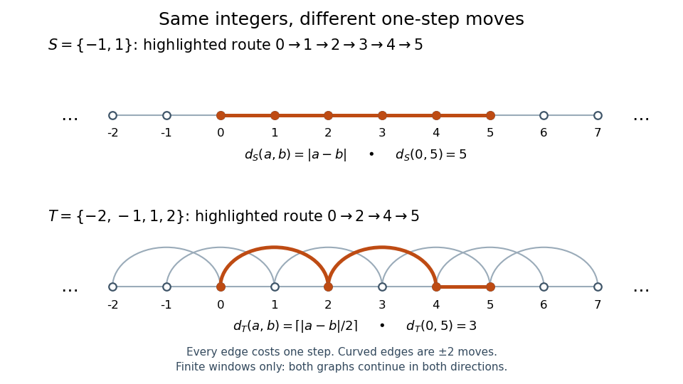
Two Cayley graphs of the integers: unit moves need five steps from zero to five; adding moves of size two needs three
. Details. 
The picture shows only a finite window of each infinite Cayley graph. By contrast, alone fails to be a generating set of a group for : it generates the subgroup . Its move graph has two connected components of a graph, the even integers and the odd integers. Within either component the graph distance is ; between different components no finite graph path exists. Adding a shortcut is different from deleting the moves needed for connectivity.
Noncharacteristic Cauchy data Created 2026-10-14 Updated 2026-10-31
For with data along , the initial curve is noncharacteristic when its tangent is linearly independent of the projected characteristic vector evaluated at the initial value of . The determinant is , up to sign. For coefficients and data this permits the inverse function theorem to invert the local characteristic parametrization and gives a unique local classical solution.
Finite-rank KdV dressing determinant 2026-10-14
Choose distinct and weights at spectral points . With and , solve . The reconstructed multisoliton solution is . Since , cyclicity of the trace gives . The Cauchy matrix is positive definite, because it is the Gram matrix of on ; diagonal similarity then proves . For one spectral point this yields .
Dual Cauchy identity for symmetric functions 2026-10-14
Apply the symmetric-function involution in one alphabet to the ordinary Cauchy identity. It changes complete generators to elementary ones and, by the dual Jacobi–Trudi identity, sends to . This proves the identity as a formal series and relates pairings with transposed Young shapes to squarefree matrix weights.
Given with , put for . The Cauchy identity for symmetric functions and Jacobi–Trudi identity give , degree by degree in the completion. For the coefficients are ; for they are .
For a holomorphic function on a neighbourhood of a closed disc, parametrize the Cauchy derivative formula on its boundary. The conjugate Cauchy integral theorem gives . Replacing in the derivative integral by therefore gives the displayed identity. The boundary real part determines every nonconstant analytic coefficient; only an imaginary additive constant is lost.
Compact object (mathematics) 2026-10-14
A compact object (mathematics) is an object whose represented Hom functor preserves filtered colimits. This preservation condition differs from the extra right-adjoint property defining a tiny object.
Adjoint functors 2026-10-14
Diagram (category theory) 2026-10-14
Projective object 2026-10-14
An object is projective when every morphism lifts through every epimorphism . Equivalently, the functor preserves epimorphisms.
Small projective object 2026-10-14
An object with the displayed property is called small projective; the term 0-presentable here uses this all-small-colimits convention. In a presheaf category, every representable presheaf has this property by the Yoneda lemma and pointwise computation of colimits. Conversely the canonical colimit presentation of a presheaf shows that the identity on such an object factors through one representable, making it a retract. If the indexing category has equalizers, a representable retract is again representable by the representable retract criterion.
There are unlisted articles, also show them or only show them.