
Bounded-input bounded-output stability 2026-10-14
Bounded-input bounded-output stability means that every bounded plant input produces a bounded plant output from zero initial state. For a causal continuous-time linear time-invariant system with a proper rational transfer function, BIBO stability is equivalent to every pole of the reduced transfer function having strictly negative real part. Cancel common factors first: an apparent denominator root may be absent from the reduced transfer function. For with , the only pole is , so the first-order low-pass filter is BIBO stable. [ref]
https://ocw.mit.edu/courses/6-241j-dynamic-systems-and-control-spring-2011/996025f6db0d90b00f11c44fc49b85f9_MIT6_241JS11_textbook.pdf. Dahleh, Dahleh and Verghese, section 15.3.1 and example 15.5: input/output versus internal stability
Internal asymptotic stability also requires every unforced internal state to decay. A canceled factor can hide a growing internal state. For example, consider the linear system of ordinary differential equationsIts zero-state transfer function can be written and has BIBO stability. Yet from zero initial conditions and a unit-step plant input, grows without bound while the plant output remains bounded. The reduced transfer function conceals that second state. Even a transfer function with no visible cancellations can be implemented with additional hidden states; its poles alone do not establish internal asymptotic stability of an arbitrary implementation.
Proper rational transfer function 2026-10-14
A proper rational transfer function is a rational function whose numerator polynomial has polynomial degree no greater than its denominator polynomial, after common factors are canceled. Every finite-dimensional continuous-time linear time-invariant system of the form , has such a transfer function . [ref]
https://ocw.mit.edu/courses/6-241j-dynamic-systems-and-control-spring-2011/996025f6db0d90b00f11c44fc49b85f9_MIT6_241JS11_textbook.pdf. Dahleh, Dahleh and Verghese, Lectures on Dynamic Systems and Control, section 15.3.1
Continuous-time frequency response 2026-10-14
The continuous-time frequency response is the frequency response of a continuous-time linear time-invariant system. From zero initial state, a BIBO stable system driven by a sustained sinusoid approaches the steady responseAny decaying initial or switching transient is separate. The modulus is the amplitude gain; the complex argument is the shift in oscillation phase. Thus evaluating a transfer function at measures both how much of an oscillation passes through and how far it lags.
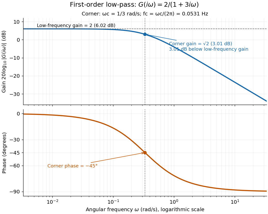
For the first-order low-pass filter, with , direct complex number arithmetic givesThe phase uses the inverse tangent branch between and . Low angular frequencies have gain close to and little lag. High angular frequencies have gain approximately and lag approaching . This is why the model is a first-order low-pass filter: it suppresses fast variation compared with slow variation. Rowell relates frequency response gain and phase to poles and then introduces Bode plots in MIT 2.004, lecture 32, sections 1 and 2.
At the corner angular frequency,For and , , the gain is , and the lag is degrees. The angular frequency is measured in radians per second; ordinary frequency is measured in hertz (cycles per second), with . Consequently the same corner is , not .
First-order low-pass filter Created 2026-10-14 Updated 2026-10-20
A first-order low-pass filter with positive constant gain and time constant obeys the ordinary differential equationThe derivative term limits how quickly the plant output follows a changing plant input. A larger time constant means slower adjustment. This standard form, with , is developed in Derek Rowell, MIT 2.004, lecture 20, section 1.1: first-order systems; the following calculation keeps the gain explicit.
Write . The Laplace transform of the derivative is , soSetting the initial condition gives the transfer function . Its single simple pole is , which has negative real part. The unforced response decays, and the input/output map has BIBO stability. The eventual gain for a constant plant input is .
For a unit step, represented by the Heaviside step function , the Laplace transform is . From zero initial condition,Take and , with dimensionless plant input and plant output. Then rises toward . After one time constant, at , it reaches , or of its final value. At , it reaches , or . These percentages describe the rise from zero, rather than an instantaneous jump to the target.
With a nonzero initial condition, the same step instead givesFor and , compare with . Their plant outputs differ by despite having the same transfer function and the same plant input. The extra exponential decay term must be supplied from the initial condition; and alone cannot determine it.
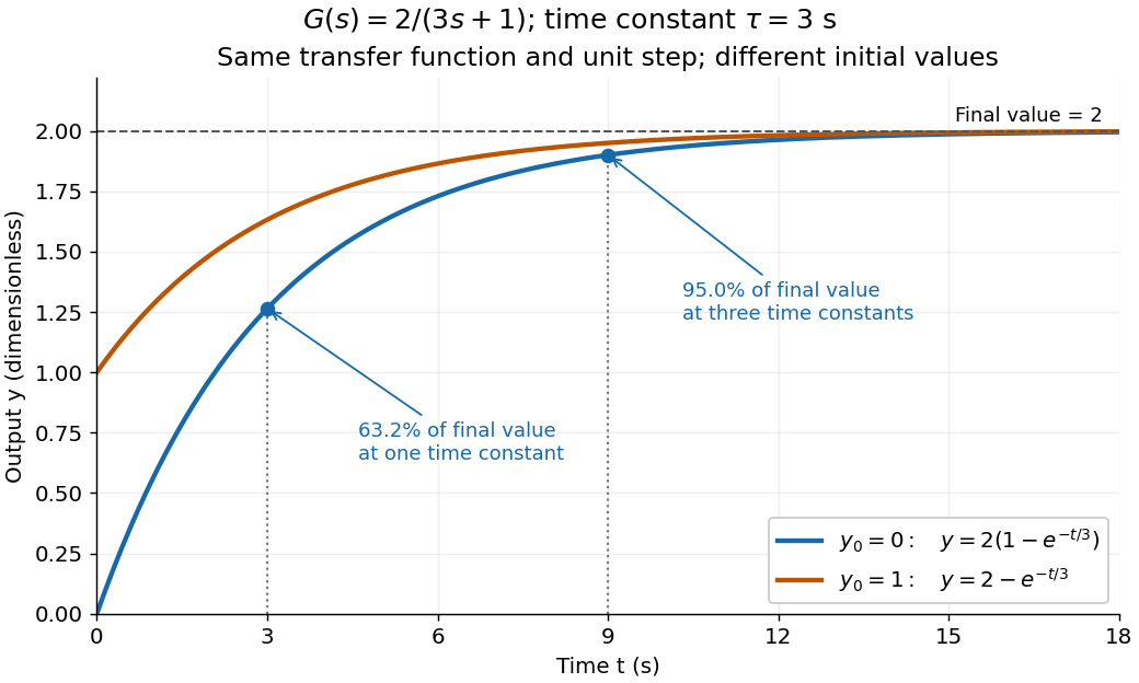
One transfer function, one unit step, two initial conditions
. The first-order low-pass filter has and time constant . The blue curve starts at and the orange curve at . The marked and levels refer to the blue curve's final value ; the two curves' difference is the decaying initial-state contribution. Details.A transcritical bifurcation need not already have its persistent branch at coordinate zero. The smooth parameter-dependent shift turns the displayed crossing of into the standard form with parameter . The crossing branches exchange dynamical stability. A mere nonsmooth relabeling of stable and unstable branches as would conceal this smooth exchange.
Applying the same measurable function to observations from two probability distributions cannot increase their total variation distance. Every output event is tested through its preimage , which was already one of the input events. ThereforeFor the four-outcome example, recording only whether the result is makes the output probability distributions identical: each is a Bernoulli distribution with parameter . The original total variation distance was , but this coarse measurement leaves zero discrepancy. Discarding information can make two sources less distinguishable.
The same contraction holds for a common Markov kernel : . On a finite set, expand , apply the triangle inequality to each output component, and use that each row of sums to one. A common randomized postprocessing step cannot increase distinguishability either.
Suppose one observation comes from either or , each with prior probability . A decision rule that chooses on an event and otherwise has success probabilityOn a finite set, choosing therefore gives . This is the equal-prior version of minimum sum of errors in a simple hypothesis test; allowing a statistical test to use an auxiliary random variable cannot improve it, because for each outcome the better of the two decisions already maximizes its contribution.
For the four-outcome example, choose after and after or , with either decision allowed after . Choosing after yields . The best success probability is 65%, with a 35% error probability. A smaller total variation distance means the two sources are harder to distinguish from one observation. Unequal prior probabilities, unequal costs, or multiple observations change this particular decision problem; the figure is not a universal bound for every experiment.
Total variation distance on a finite set 2026-10-14
Consider the probability mass functions and on the finite set . Their difference is . ThusThe event attains this difference: and . Combining and gives the same absolute discrepancy with the opposite sign. Adding to either event changes nothing, because its probability mass agrees under both probability distributions.
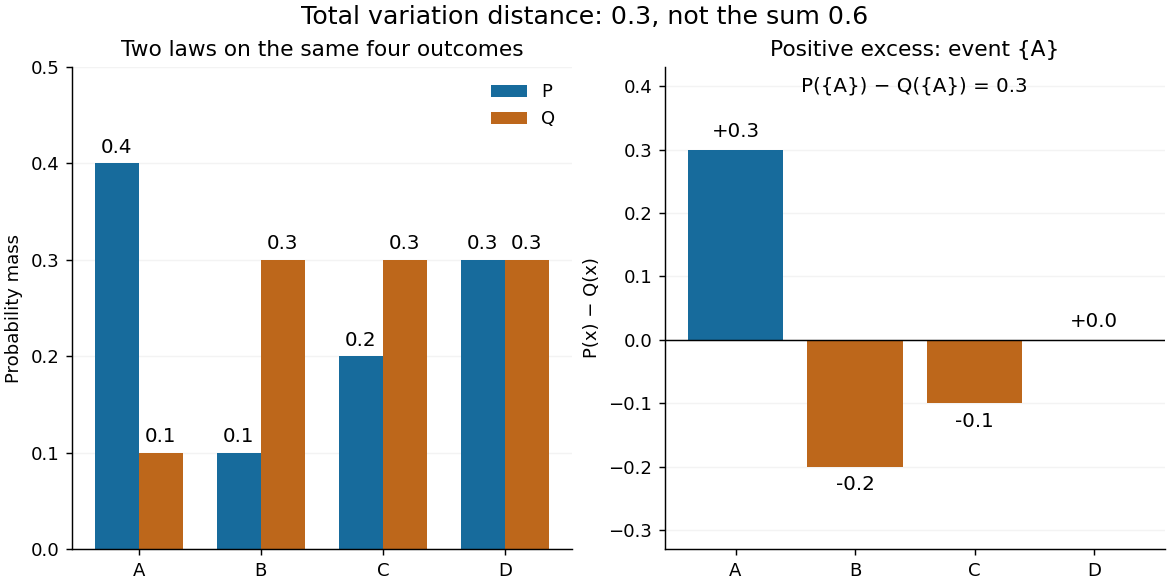
The factor is necessary because : every unit of excess probability mass must match a unit of deficit. For any event, including a negative term cannot increase its signed discrepancy, while omitting a positive term cannot increase it either. Therefore attains the positive maximum. This is a short way to compute an apparent optimization over subsets using one pass through .
For probability density functions relative to the same measure , the corresponding identity is . Such densities can always be taken as Radon-Nikodym derivatives relative to . Beware the notation: the total variation norm of a measure applied to the signed measure equals . A formula using that norm without its factor is using a different normalization.
Torsion balance zero drift 2026-10-14
Torsion balance zero drift is slow motion of the unloaded reference angle during a measurement. If the torsion constant remains fixed, a constant applied torque gives . For two equal and opposite applied torques measured at the same reference zero, their equilibrium angles differ by . A stable offset cancels; a changing zero contributes and does not cancel automatically.
A simple symmetric sequence makes the limitation explicit. Let be settled equilibrium angles for applied torques at equally spaced times . If the unloaded zero is linear in time, , and and remain fixed, thenThe arithmetic average of the outer zero values equals the middle zero, so both the constant offset and linear drift cancel. Curved zero motion, unequal time spacing, changing torsion constant, changing signal strength, or unsettled oscillations violate these assumptions. This is an algebraic control example, not a claim that every torsion balance follows a linear drift law.
Torsion constant Created 2026-10-14 Updated 2026-10-18
The torsion constant, or torsional spring constant, is the positive restoring torque per unit twist angle of a complete suspension in its linear elasticity range:Its SI unit is . The minus sign describes restoration toward the untwisted orientation. The derivative specifies a local stiffness if the response is not globally linear; using one constant over a finite range additionally requires a straight calibration curve. Return to the same zero after unloading tests recoverable elastic deformation; repeat loading in both directions to check whether the response depends on its previous loading. Staying below permanent deformation is necessary, but does not alone prove proportionality between torque and twist.
For an ideal uniform circular wire of length , radius , and shear modulus , the filament torsional stiffness is , with polar second moment of area . Uniform twist gives as the twist per unit length, soHere is stored elastic energy. Doubling the wire's radius multiplies the ideal torsion constant by ; doubling its length halves it. This explains why a long thin fiber is useful for weak torque measurement. The formula assumes linear elasticity with uniform material and circular section; it does not calibrate arbitrary ribbons, clamps, or a compound suspension. Within this ideal model, the equipartition theorem predicts an equilibrium thermal mean-square angular displacement , where is the Boltzmann constant and the uniform absolute temperature. A softer suspension magnifies both the signal and its thermal fluctuations.
Static calibration supplies known torques without assuming the unknown interaction being measured. Apply a known perpendicular force at lever arm , record the change from the unloaded twist, and useSeveral positive and negative settings test proportionality; fit the slope of applied torque against twist and retain a possible intercept. A nonzero intercept must not be silently absorbed into the slope. Convert degrees to radians before reporting . PASCO's procedure turns the Coulomb balance on its side and adds small known masses to generate a gravitational weight at the sphere's lever arm, returning the rod to its index mark by turning the dial. Its tabulated coefficient is force per degree: multiply by the lever arm and to obtain our torsion constant. [ref]
https://cdn.pasco.com/product_document/Coulombs-Law-Apparatus-Manual-ES-9070.pdf. Bruce Lee, PASCO ES-9070 manual, pp. 9–10: mass calibration and force-per-degree convention
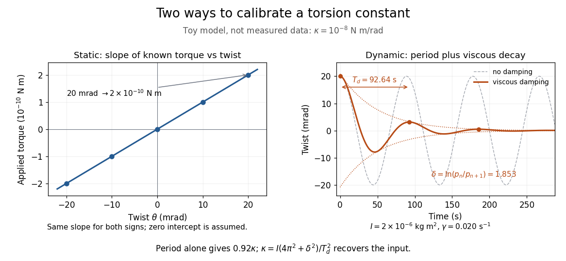


The figure's ideal static calibration uses : an applied torque of gives . Both signs lie on the same straight line. The plotted points are calculated examples, not experimental observations; they cannot demonstrate a real fiber's linearity.
Dynamic calibration instead measures the oscillation period with known total suspended moment of inertia . For negligible damping, small free oscillations about a fixed reference obey simple harmonic motion:Include the rod, mirrors, and any attachments in unless their contributions are demonstrably negligible. Keep the applied torque absent or independent of angle. If an external torque has derivative at equilibrium, linearization gives effective stiffness : timing alone then measures that combination, and stability requires . A constant applied torque merely shifts equilibrium. Non-negligible damping changes the measured period; damped torsional oscillation gives a correction under a specified damping model. Agreement between static and dynamic calibrations is a useful check on the assumed moment of inertia, reference stability, and restoring law, rather than a reason to ignore their assumptions.
Knaster-Kuratowski-Mazurkiewicz lemma 2026-10-14
For a simplex with vertices indexed by , let closed sets have the property that every face spanned by an index set lies in . Then is nonempty. The triangle KKM lemma is a two-dimensional covering formulation of this simplex-intersection principle.
Normal space 2026-10-14
A topological space is normal when every two disjoint closed subsets have disjoint open neighbourhoods.
Dense set 2026-10-14
Topological disc 2026-10-14
An -dimensional topological disc is a space homeomorphic to a Euclidean ball in , with its open or closed convention specified. A closed disc is homeomorphic to . The planar disk is the Euclidean two-dimensional instance, rather than the whole abstract topological class.
Disk (mathematics) 2026-10-14
A planar Euclidean disk consists of the points within a fixed radius of a centre, with either the open or closed boundary convention. The closed disk centered at the origin is and has area . It is the two-dimensional closed Euclidean ball; the general closed disc may have any dimension.
Closure (topology) 2026-10-14
The closure of a subset of a topological space is the smallest closed set containing . Equivalently, it is the intersection of all closed sets containing , or the set of points whose every neighbourhood in meets . The notation makes the ambient topological space explicit. This definition works without a metric or any appeal to sequences. [ref]
https://math.mit.edu/~hrm/palestine/munkres-topology.pdf. James Munkres, Topology, closure and interior of a set
For in the usual real line, : every neighbourhood of meets , while a point outside has an open ball disjoint from . Passing to the closure adds the missing endpoint and retains all original points, including isolated points when present. In general, the closure is together with its limit points; its individual points are the adherent points of .
The closure turns an arbitrary subset into a closed set with no unnecessary added points. It satisfies and ; a subset is closed exactly when . In a metric space, exactly when some sequence of points of has limit of a sequence : choose its th point in . For a general topological space, keep the neighbourhood definition; sequences need not detect every point of the closure.
Extremally disconnected space 2026-10-14
A topological space is extremally disconnected when the closure of every open set is open. This concerns open sets, not arbitrary subsets. In particular, a nonisolated singleton in a Hausdorff space is closed but not open, so its closure gives a counterexample to that stronger condition.
Symmetric product 2026-10-14
The th symmetric product of a space is , where the symmetric group permutes the factors. Its points are unordered -tuples, with repetitions allowed. If is a Riemann surface, elementary symmetric functions in local complex coordinates make its symmetric product a smooth complex manifold, including along the locus of repeated points. A collection of disjoint circles in gives a product torus in this symmetric product.
Lower limit topology 2026-10-14
The lower limit topology on has basis of a topology . Every such nonempty interval contains a rational, so this topological space is separable. Its topology is finer than the usual Euclidean topology; the one-sided basic neighbourhoods allow its square to have an uncountable discrete antidiagonal.
On an infinite set, the family consisting of all finite subsets and the whole set need not be closed under arbitrary unions. On , the union of the singleton subsets of is infinite and proper, so this family is not a topology. It must not be confused with the cofinite topology, whose proper open sets have finite complements.
There are unlisted articles, also show them or only show them.