
Fermion flow 2026-10-14
The arrow on a charged-fermion line in a Feynman diagram tracks fermion-number flow and fixes the order of the gamma matrices between external Dirac spinors. For an external particle it agrees with the particle direction; for an external antiparticle it is opposite to the antiparticle direction. It therefore need not point along the assigned four-momentum of every external leg.
Feynman integral Created 2026-10-14 Updated 2026-10-18
A Feynman integral is the momentum-space integral associated with a Feynman diagram: each independent loop momentum is integrated with measure , and propagators, vertex numerators and momentum conservation determine the integrand. Its definition also requires a pole prescription and, when divergent, a regularization in quantum field theory. Feynman parameters combine propagator denominators and permit shifts of loop momenta. A massless two-propagator example is , with its causal prescriptions understood. Subtracting local counterterms turns a regulated diagram into a finite contribution to a renormalized amplitude.
Polarized fermionic Fock space Created 2026-10-14 Updated 2026-11-05
An orthogonal projection splits a one-particle Hilbert space into empty and filled modes. Take completed exterior Fock spaces of empty particles and of holes in the filled modes, with the graded tensor product enforcing the canonical anticommutation relations between both factors. The vacuum is killed by particle annihilation in and by particle creation in . Only finite particle-hole excitations are needed for a dense basis. Normal ordering subtracts the filled-vacuum expectation from bilinear observables.
Let , , and let be a normalized eigenstate of with , where is the Clifford vacuum. Acting with the supercharge differentiates only its wavefunction:The normalized partner is . Indeed , and ; acting with again returns times the original state. The expression at is interpreted by the regular extension of the original state. Although its coefficient depends only on , its degree-one components contain the radial unit vector.
Pépin's test 2026-10-14
For , Pépin's test says that the Fermat number is a prime number exactly when the displayed modular congruence holds. Modular exponentiation evaluates it by exponentiation by squaring without constructing the enormous ordinary power. The index restriction excludes , where the base itself is divisible by the candidate.[ref]
For a proof outline of sufficiency, any prime factor of a passing candidate gives multiplicative order exactly , a power of two: its half-power is , rather than . Fermat's little theorem forces , so , and hence . Conversely, for a prime candidate, ; quadratic reciprocity and Euler's criterion give the required half-power. At , the check is .
Distinct Fermat numbers are coprime 2026-10-14
If , a common divisor of and divides both , by the Fermat number product identity, and . It therefore divides two. Both Fermat numbers are odd integers, so their greatest common divisor is one. Each term's prime factors are consequently different from the prime factors of every other term.
Feigenbaum attractor Created 2026-10-14 Updated 2026-11-05
For the normalized Feigenbaum map, put and defineThe Feigenbaum attractor is the nested intersection . Each level interval has two children, and the largest interval length tends to zero. Consequently every compatible infinite binary address selects one point of this Cantor set.[ref]
At level , the intervals are visited cyclically: the label changes from to modulo . Expressing in binary therefore turns iteration on into the dyadic adding machine. One adds one with carries, rather than discarding the first symbol as in a full shift. For example, addresses written with the least significant digit first begin .
There are geometric pieces at depth , but those pieces are visited in a cycle. Counting them does not make the time evolution a two-symbol full shift. The Feigenbaum geometric potential uses this depth to study spatial contraction and Hausdorff dimension.
Feigenbaum geometric potential Created 2026-10-14 Updated 2026-11-05
The Feigenbaum geometric potential is a bounded negative symbolic potential encoding the lengths of nested intervals of the Feigenbaum attractor. In an appropriate binary coding,and changing only the distant tail of an address changes by an exponentially small amount. For odd interval labels, a sum along reversed address prefixes satisfieswith a bound independent of the depth and address. Even-label intervals have lengths comparable to neighboring odd-label intervals. These uniform estimates connect geometric lengths with thermodynamic formalism.[ref]
Feigenbaum universality and the thermodynamic formalism by E. B. Vul and others. Thermodynamic description of the period-doubling geometry
[ref]Multifractality of the Feigenbaum attractor and fractional derivatives by Uriel Frisch and others. Section 2.1, equations (8)–(14): bounded potential, decaying variations and interval-length comparisons
The bounded logarithmic error is important. For fixed real , exponentiation givesAfter summing and taking , the error is at most , which vanishes. Thus geometric partition sums and symbolic partition sums give the same limiting topological pressure. The almost-additive partition-function limit supplies existence under the bounded-distortion hypotheses; bounded negative potentials give a strictly decreasing pressure.
This potential measures geometric contraction across partition levels. It is not an unbounded derivative potential evaluated at the critical point, where , and partition depth is distinct from elapsed orbit time.
Delayed cursor feedback experiment 2026-10-14
Can feedback delay change correction timing even when the physical task stays the same? Susilaradeya and colleagues tested this in a human tracking experiment. Participants pressed with both index fingers against fixed force sensors; the two forces controlled a screen cursor along two diagonal axes. A target moved in slow circular motion, usually at rotations per second. The researchers sampled the forces at samples per second and inserted an additional delay of , , , , or milliseconds before displaying the cursor. Each trial lasted seconds; the trials included per delay, in pseudorandom order. [ref]
https://pmc.ncbi.nlm.nih.gov/articles/PMC6453565/. Susilaradeya et al., Extrinsic and intrinsic dynamics in movement intermittency (2019), figure 1 and human task methods
The readout was fluctuation in cursor angular velocity, analyzed by Fourier transforms over approximately seconds from the middle of each trial. The principal peak was around hertz without added delay, around hertz with milliseconds, and around hertz with milliseconds. Thus changing observation timing changed the timing of corrective motion. [ref]
https://pmc.ncbi.nlm.nih.gov/articles/PMC6453565/. Susilaradeya et al., results: submovement frequencies are affected by feedback delays
This is an empirical motivation for taking stale observations seriously. Human feedback control includes prediction and other dynamics; these observations do not measure in the ideal integrator model or test its boundary.For the constant-coefficient model with and , the zero equilibrium point is asymptotically stable if and only if . For positive , perturbations are measured by the supremum norm of the initial history of delayed feedback; in the stable regime, every continuous history produces a solution tending to zero. At equality, nondecaying sinusoids prevent asymptotic stability. For , growing oscillatory solutions exist. These statements concern this ideal linear time-invariant system, rather than an arbitrary controlled plant. The corresponding linear equation and its threshold are developed in Cain and Reynolds, section 6.4, pages 174–177.
Substitute the exponential function , allowing a complex number . The characteristic equation isFor positive feedback delay this is not a characteristic polynomial: it has infinitely many roots. A root's real part determines growth or decay of its exponential mode, and its imaginary part determines the angular frequency. To find the first boundary, set with and use Euler's formula:The smallest positive crossing is and . Thus at the complex conjugate roots are . In fact, with the matching initial history of delayed feedback,solves the delay differential equation exactly: a quarter-cycle feedback delay turns the past displacement into precisely the current derivative. Its cycle lasts . The amplitude is arbitrary; this linear model does not select a finite-amplitude oscillation.
The roots cross toward growth as feedback delay increases. Differentiating the characteristic equation at fixed givesThis calculation identifies the direction of the first destabilization. The full threshold also requires ruling out earlier unstable roots: if with and , the characteristic equation implies and , hence . A real nonnegative root is impossible because there. This supplies the geometric reason the threshold is a quarter-cycle rather than an arbitrary fitting constant.
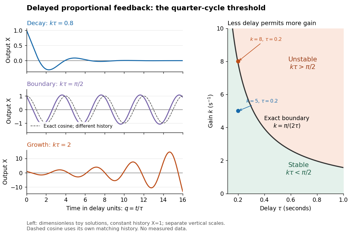
Feedback delay separates decay, persistent oscillation, and growth
. Left: numerical solutions with the same constant initial history of delayed feedback on , plotted against for , , and . The middle trajectory includes a transient because this history is not a pure sinusoid; the dashed curve is a separate exact solution with history . Each row has its own vertical scale. Right: the exact boundary for positive feedback gain and feedback delay. Toy responses are not measured data. The generator uses the classical fourth-order Runge-Kutta method with linear interpolation of delayed values and , checked against a separately evaluated exact finite sum and two coarser steps. Details.
The tradeoff is concrete. Without feedback delay, increasing shortens the exponential decay time constant . With known , the same proportional control must satisfy . For , the threshold is : is stable and is unstable. A design close to the boundary leaves little room for additional feedback delay; reducing or reducing measurement latency increases that room. The zero-delay time constant is only a comparison scale, not the decay time of the delayed response. Frank discusses the gain–delay compromise in Control Theory Tutorial, section 13.4 and figure 13.3.
Initial history of delayed feedback 2026-10-14
For positive feedback delay , an initial condition at a single instant is insufficient. Prescribe a continuous function throughout : for , the derivative depends on . A right derivative at is understood; the earlier history need not itself obey the subsequent control law. Once this first interval is computed, it supplies the delayed values for the next interval. This successive integration is the method of steps for a delay differential equation. [ref]
https://math1um.github.io/Teaching/cain-reynolds-odes.pdf#page=174. John W. Cain and Angela M. Reynolds, Ordinary and Partial Differential Equations, sections 6.1 and 6.2: history and the method of steps
For the constant initial history of delayed feedback , direct integration givesFor , , the plant output crosses zero at , while its measured output remains positive until . At , the delayed command therefore increases the magnitude of the actual deviation. This short exact calculation explains the first diagram without relying on a numerical approximation.
Fatou component 2026-10-14
A Fatou component is a connected component of the Fatou set of a rational map. It is open. A rational map sends each Fatou component onto another one: complete invariance of the Fatou set puts it inside the inverse image of the target component; its maximal connectedness makes it one full inverse-image component. Restricting the globally proper sphere map to such a component is proper, since the inverse image of a compact subset intersected with the component is closed in a compact set. Its image is both open and closed in the connected target component, hence the whole target. A component is periodic if some iterate returns it to itself.
Under random mating and Hardy-Weinberg equilibrium, label each parental allele by whether it is transmitted. Let and be the transmitted/untransmitted pairs of two parents. Before ascertainment all four draws are independent with population frequencies . If offspring disease weights the transmitted pair by , thenThe transmitted pair is an affected-case genotype and the untransmitted pair a population family pseudo-control genotype under this homogeneous model. For unordered genotypes, compatible labelled transmissions must be summed. Conditioning on parental genotypes instead removes nuisance population frequencies and gives the usual transmission disequilibrium test.
// Target: statistical-modelling.bigb
A falling free surface does not instantaneously dry previously wetted rigid walls. Thin films remain above the bulk liquid and drain under the component of gravitational acceleration parallel to the walls. For a film of thickness over a wetted distance , falling film flow gives a speed of order , hence at late times for an order-one wall angle. These films can be visible in a cross-section while holding asymptotically negligible volume. In a V-shaped channel gravity current, local bulk depth falls only as ; at a fixed nonzero station with a finite previous maximum wetted height, film volume decays as while bulk-sectional volume decays as . Thus the film does not change the leading spreading law.
Two-layer falling film of equal-density viscous fluids Created 2026-10-14 Updated 2026-10-18
Let the lower fluid have thickness and viscosity , and the upper fluid thickness and viscosity , with common density . For steady flow down a plane inclined at angle , set , . The common hydrostatic pressure is . No slip at the wall, continuous velocity and shear stress at , and zero upper surface shear give and . These follow by integrating in each layer. The stress applied to the lower fluid equals the downslope weight of the upper layer, independent of its viscosity; the upper viscosity affects its shear rate but not that transmitted stress.
Exponent vector Created 2026-10-14 Updated 2026-11-05
Relative to an ordered factor base , a positive integer has exponent vector . Multiplication of such integers adds their exponent vectors. Reducing every coordinate modulo two gives the parity vector used to find congruences of squares. The ordering and any sign coordinate must be used consistently across all rows.
The supergravity F-term potential on the inflationary branch has the displayed exact form. Its expansion is , so the inflaton quadratic mass cancels at tree level for this canonical model. For its derivative is ; the branch is therefore a transverse valley, not a stationary supersymmetry-breaking vacuum.
In the small-field global approximation, the waterfall fluctuations on have the displayed masses. One becomes negative when , driving the fields towards the supersymmetric vacuum branch. In the canonical supergravity model, the exact masses follow from expanding the exponential and Kähler-covariant derivatives; their Planck-suppressed corrections should not be discarded unless the corresponding field and symmetry-breaking scales are small.
For nonzero and , these field values give and all Kähler covariant derivatives of a superpotential zero, hence zero supergravity auxiliary fields and zero vacuum energy. With only the supplied chiral fields, the product condition gives a complex vacuum manifold rather than one isolated point. A specified gauged opposite-charge symmetry can add a D-flatness condition and a gauge quotient, but no such gauge sector should be invented from the field labels alone.
Let be an integer and let be independent and identically distributed random variables with an exponential distribution of rate . Their sample maximum is nonnegative. Substituting the exponential distribution's cumulative distribution function into the distribution functions of independent minima and maxima gives the exact lawFor example, at each observation is below the threshold with probability , but all observations are below it with probability . Thus an individual observation's median becomes an increasingly unlikely upper bound for the whole batch. The general order statistic density in Siegrist's treatment, with , also gives this law on integration. [ref]
https://www.randomservices.org/random/sample/OrderStatistics.html. Siegrist, Random Services: exponential order statistics
.Solving gives the exact quantile function, for ,In a toy model with , the median maximum is seconds for , seconds for , and seconds for . All three use the exact distribution function; the increase comes from taking a maximum over more observations. The case connects to the existing maximum of two exponentials as a scaled sum.
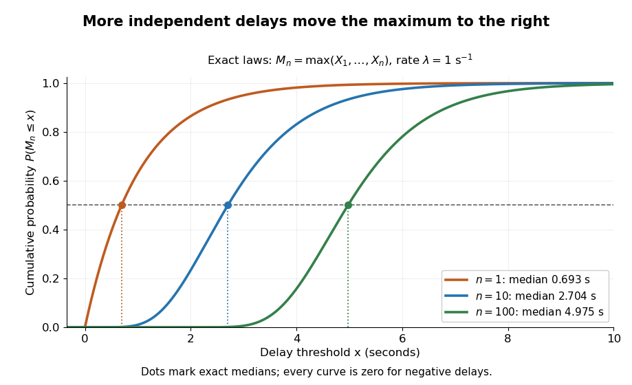
Exact cumulative distribution functions of exponential sample maxima, with rate one per second and median markers
. Details. 
The Gumbel distribution explains the logarithmic shift visible here: after subtracting and measuring deviations in units of , the distribution functions approach one fixed shape. The next derivation makes that convergence in distribution explicit.
There are unlisted articles, also show them or only show them.