
Diagram (category theory) 2026-10-14
Projective object 2026-10-14
An object is projective when every morphism lifts through every epimorphism . Equivalently, the functor preserves epimorphisms.
Small projective object 2026-10-14
An object with the displayed property is called small projective; the term 0-presentable here uses this all-small-colimits convention. In a presheaf category, every representable presheaf has this property by the Yoneda lemma and pointwise computation of colimits. Conversely the canonical colimit presentation of a presheaf shows that the identity on such an object factors through one representable, making it a retract. If the indexing category has equalizers, a representable retract is again representable by the representable retract criterion.
Morphism in a category 2026-10-14
A categorical morphism is an arrow with a specified source and target in a category. An arrow composes with to give . Composition is associative, and every object has an identity arrow acting as a unit. A functor preserves the sources, targets, identities and compositions of these arrows. In a locally small category, the arrows between fixed objects form a hom-set.
Duality (category theory) Created 2026-10-14 Updated 2026-11-05
Reversing the arrows in a categorical statement produces its dual statement. A theorem holding for all categories therefore has a dual theorem obtained by applying it to the opposite category; for example, categorical limits are exchanged with colimits.
Transition state theory Created 2026-10-14 Updated 2026-10-20
Transition state theory relates an elementary reaction's rate constant to a Gibbs energy of activation. The Eyring expression used in the catalyst example assumes every passage counted at the transition state succeeds. More generally, a factor accounting for unsuccessful passage multiplies it. Comparing barriers alone gives the quoted speedup only when the remaining prefactors agree. Free-energy profiles can depend on temperature, so the example's values at do not determine a temperature curve. See the IUPAC Gold Book: transition state theory.
Hadamard space Created 2026-10-14 Updated 2026-11-05
A Hadamard space is a complete CAT(0) space. Equivalently, it is a complete metric space in which every pair has a midpoint satisfyingfor every . A midpoint means . Substituting a second midpoint for forces their distance to be zero, so the midpoint is unique.
Iterating midpoints defines the joining geodesic first at dyadic parameters. Completeness then supplies its points at every real parameter. The midpoint inequality extends by this approximation to the Hadamard squared-distance inequality, and hence to Euclidean triangle comparison. In particular, closed balls have geodesic convexity.
The completeness condition belongs in both formulations. The rational numbers with the usual distance have all rational midpoints and satisfy the displayed inequality, but are incomplete. A full real-parameter geodesic from zero to one would require irrational points. Thus the midpoint inequality alone does not make that space a Hadamard space.
For an integral domain with fraction field , realize Cartier divisors as invertible fractional ideals, with local divisor equation corresponding to the ideal . This is the convention. The maps in the displayed exact sequence are unit inclusion, , and . A principal fractional ideal is trivial as a divisor exactly when its generator is a unit. An invertible fractional ideal is trivial in the Picard group of a ring exactly when it is principal. Every rank-one projective module embeds in and produces an invertible fractional ideal, proving surjectivity. Local multiplication identifies with , so these are group homomorphisms.
Pullback of a Cartier divisor 2026-10-14
For a morphism of varieties , pull back local defining rational functions of a Cartier divisor whenever they remain nonzero on each component of . Their ratios remain regular units, defining . Equivalently, pull back the associated line bundle and its rational section. A dominant morphism always permits this construction.
Affine section of a planar set Created 2026-10-14 Updated 2026-10-25
For and a nonzero direction , its affine section is the inverse image of under the line parametrization . The resulting set is a subset of the parameter line, so changing a parametrization can change the section by translation or scaling. The four real parameters can be encoded by a single real using real-number pairing by separated digits. Thus no fixed planar set can realize every real subset as a section, by Cantor's theorem.
Quadrant (plane geometry) Created 2026-10-14 Updated 2026-10-18
The two coordinate axes divide a Cartesian coordinate system in the plane into four open quadrants, distinguished by the signs of their coordinates. The positive quadrant is the first quadrant.
Stoichiometric imbalance in step growth 2026-10-14
For a strictly bifunctional feed, label the limiting functional groups , set , and define as in functional-group conversion in step growth. The initial molecule count is , and each intermolecular join consumes one and one . ThusThis version of the Carothers equation uses limiting-group conversion, not the fraction of all groups reacted.[ref]
As an original finite example, mix monomer molecules with monomer molecules. Then and . At , joins leave molecules, giving . At , joins leave five chains and ten unreacted groups; every chain has two ends, and . Continuing to wait cannot remove the missing- constraint within this model.
For , complete limiting-group conversion gives the ceiling . Reaching a target therefore requires , even before considering incomplete conversion. For , . Equality requires ; any lower conversion demands closer balance. The imbalance is measured relative to the initial number of groups, not relative to the total number of groups. A monofunctional impurity changes the initial groups-per-molecule count, so it cannot be inserted into this strictly bifunctional formula by retaining an unexamined .
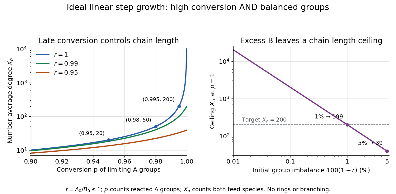
Carothers equation sensitivity to limiting-group conversion and initial stoichiometric imbalance in step growth
. Original analytic model curves with logarithmic vertical axes. Left: and the balanced example points. Right: versus , the initial excess- fraction relative to . These are ideal linear no-ring calculations, not fits to the polyurethane study. Details.
Chow-Rashevskii theorem 2026-10-14
On a connected manifold, a smooth bracket-generating family of vector fields connects every pair of points by a piecewise smooth horizontal curve. For a free step-N nilpotent Lie group, this says that every group element is the path signature of a sufficiently regular path. In the planar step-two case, a closed rectangle prescribes the signed area and a following straight segment prescribes the displacement.
Carleson box 2026-10-14
A boundary neighborhood over an arc of the unit circle, with radial depth equal to its normalized angular length . Changing that depth by any fixed positive factor gives an equivalent Carleson measure condition. Large arcs and central mass can be handled separately by finitely many fixed neighborhoods covering the unit disc.
Carleson embedding theorem on the disk 2026-10-14
A positive Borel measure on the unit disc satisfies for every H1 space on the unit disk function exactly when it is a Carleson measure, with comparable optimal constants. The normalized squared Cauchy kernel tests necessity. For sufficiency, the boundary shadow of every point with lies inside a component arc of . The geodesic-cap and Carleson-box comparison bounds the measure of each shadow region by its component length, giving . The layer cake representation and H1 non-tangential maximal inequality on the disk give the embedding. The broader kernel and covering mechanism is discussed in Terence Tao's harmonic-analysis notes, Exercise 2 after Lemma 4.1; the analytic endpoint here uses the fractional-power argument just given.
Zhu, Miao, Xu and Cao's 2007 experiment drove a triangular metal frame electromagnetically with a sinusoidal generator. In a roughly -deep, temperature-regulated pool, it produced nearly plane capillary waves. A laser illuminated the surface obliquely; the moving ripples acted as a reflection diffraction grating. One split beam monitored laser stability, while a CCD recorded diffraction orders on a screen away. An air-supported optical table reduced ambient vibration. [ref]
https://www.eg.bucknell.edu/~phys310/skills/papers/paperX_full.pdf. Zhu et al., Measurement of the dispersion relation of capillary waves by laser diffraction, American Journal of Physics 75 (2007), §II.A, p. 896; DOI 10.1119/1.2750379
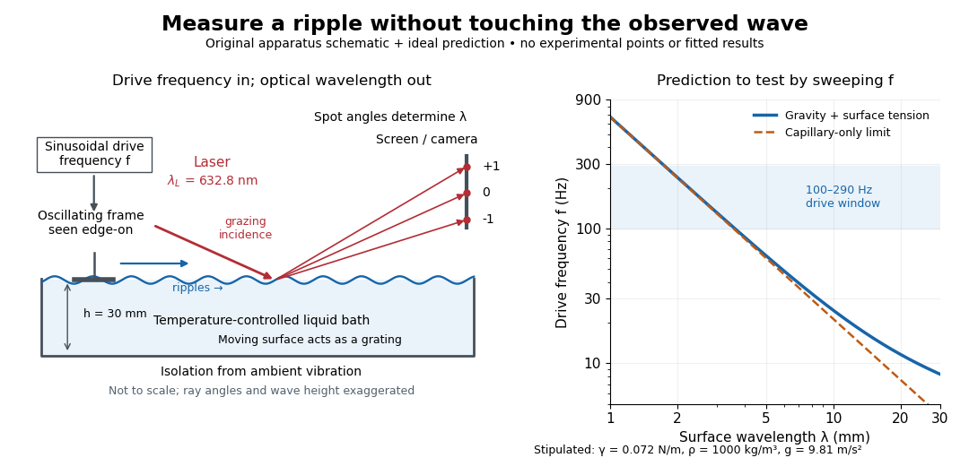

The frequency sweep was – in steps, using distilled water and kerosene at . For each setting they averaged at least three measurements of first-order spot separation. Known optical geometry and the grating equation yielded ; generator readings yielded . Agreement with the predicted log–log slope tests the capillary law, and its intercept gives surface tension if mass density is known. The authors identify surface contamination as a major error source; noncontact optical detection reduces additional disturbance. [ref]
https://www.eg.bucknell.edu/~phys310/skills/papers/paperX_full.pdf. Zhu et al., §§II.B–III, equations (6)–(8), pp. 897–898
The optical measurement can be understood from the grating equation. Let be the laser wavelength, the incident grazing angle above the mean surface, and the outgoing grazing angle of diffraction order , with the sign of chosen so thatThus calibrated spot positions determine outgoing angles, which determine the ripple wavelength , independently of the mechanical dispersion relation. This optical geometry treats the surface as a reflection diffraction grating at the laser wavelength. [ref]
The inferred surface tension in the full deep-water model isThis formula makes useful experimental controls explicit. Measure mass density at the sample's temperature; check depth with ; keep the driven wave amplitude small enough that ; and distinguish from angular frequency . For the stipulated parameters, the – window corresponds to calculated wavelengths about – and – at . Depth corrections are negligible here, but the gravity contribution is about – of the capillary contribution. These are ideal predictions, not digitized results from the experiment.
Omitting gravity would infer , biasing surface tension upward. In the capillary limit, the differential estimate also shows why careful spot-spacing calibration matters. A clean surface and weak viscosity are modeling assumptions: appreciable damping, surfactant stresses or large wave amplitudes call for additional physics. The experiment tests the short-wave regime; its drive window does not establish the crossover or the long-wave surface gravity wave limit.
Gravity-capillary wave Created 2026-10-14 Updated 2026-10-20
A gravity-capillary wave has restoring contributions from both gravity and surface tension. Consider an initially resting, horizontally unbounded liquid layer of constant depth , with uniform mass density , incompressible flow, inviscid flow and irrotational flow. The upper gas exerts constant pressure and has negligible inertia. Assume a clean interface with constant surface tension : no surfactant stresses, imposed current or wind. The wave amplitude must satisfy and , so linearized boundary conditions apply. Deep water means , rather than a particular depth in metres. [ref]
https://www.ocw.mit.edu/courses/18-354j-nonlinear-dynamics-ii-continuum-systems-spring-2015/6163837c5efa5d6ed969e535ec8f890c_MIT18_354JS15_lectureNotes.pdf. Brenner, Peacock, Stocker, Reis and Dunkel, MIT Nonlinear Dynamics II, §23.1, pp. 105–106
Let be the undisturbed free surface, with liquid below it. Potential flow gives a velocity potential with , and incompressible flow gives the Laplace equation. The linearized kinematic boundary condition for a free-surface graph and the Unsteady Bernoulli equation, including gravity and the Young–Laplace equation, giveHere is the interface displacement; the signed small-slope pressure jump is . A wave crest has , so its capillary pressure is positive. Choose a right-travelling Fourier mode of positive wavenumber and angular frequency :The factor decays into the deep liquid, satisfies the Laplace equation, and makes at . Substituting in the dynamic boundary condition leavesThis derivation displays the two restoring contributions with the same sign. Dimensional analysis also checks the result: has units , so both and have units . [ref]
https://www.ocw.mit.edu/courses/18-354j-nonlinear-dynamics-ii-continuum-systems-spring-2015/6163837c5efa5d6ed969e535ec8f890c_MIT18_354JS15_lectureNotes.pdf. MIT Nonlinear Dynamics II, §23.1, equations (547)–(551): boundary conditions and dispersion
At finite depth, a flat impermeable bottom at requires . Replacing by the normalized vertical factor makes the surface ratio . Eliminating the mode amplitudes then givesThus the same model supplies its own depth check: use the deep-water formula only when is sufficiently close to one for the required accuracy. For example, reduces by about relative to deep water, while reduces it by about . These percentages are calculations from this factor. [ref]
In deep water the phase velocity magnitude follows a wave crest, while the group velocity magnitude follows the wave envelope of a narrow wave packet. Differentiating the positive-frequency dispersion relation givesFor , the surface gravity wave limit has . For , the deep-water capillary-wave dispersion relation has : a wave crest slips backward relative to the faster wave envelope, even while both advance. Neither speed is the oscillating fluid element's own velocity. [ref]
There is a particularly neat coincidence at the crossover. Differentiate : its unique minimum is at , exactly where the restoring terms are equal. ThereforeFor the stipulated parameters in capillary length, the minimum is . At , direct substitution gives , and . This short wavelength is capillary dominated, but its group velocity is still slightly below the pure-capillary ratio because gravity has not vanished.
Weighted binary-sequence metric 2026-10-14
On this sum is a metric, since each summand obeys the triangle inequality and a zero sum forces coordinatewise equality. A prefix cylinder set fixing the first coordinates contains the open ball of radius about each of its points and has diameter at most . These bounds show that the metric topology equals the prefix cylinder set topology, the usual Cantor space topology.
Gauge reduction of the Maxwell Hamiltonian Created 2026-10-14 Updated 2026-11-05
For a spatial potential with , the Maxwell Lagrangian gives and . Its Hamiltonian is . Preserving the temporal momentum first-class constraint gives the Gauss law constraint in gauge theory. In free space, Coulomb gauge and decay at spatial infinity set and leave only transverse modes. The reduced Dirac bracket uses the projector , so quantization gives the transverse equal-time commutator and the positive Hamiltonian displayed above.
Canonical momentum sign in the affine particle action Created 2026-10-14 Updated 2026-10-18
For the affine action with signature , differentiating with respect to velocity gives the displayed canonical momentum. Future-oriented proper time in a conformally flat metric yields , whereas the conventional future-directed mechanical momentum has . Changing the action's overall sign interchanges these canonical labels but leaves its classical geodesics unchanged. Both labels are conserved by spatial translation invariance, and either gives the same physical momentum magnitude proportional to . The sign should be stated when comparing a worldline canonical covector with a positive-frequency field-mode label.
There are unlisted articles, also show them or only show them.