
In , any set of distinct conjugates freely generates its subgroup. Combine adjacent powers of the same conjugate in a reduced word. After expansion, distinct successive indices leave nonzero intervening powers of , and the intervening nonzero powers of cannot cancel in the free product . The same argument works with interchanged and for finite or countably infinite sets of indices.
Finite-index image of a free-group endomorphism is surjective Created 2026-10-14 Updated 2026-10-31
An endomorphism of has image generated by at most elements. If this image has finite index , the Nielsen–Schreier formula gives rank . Its abelianization requires at least that many generators. For , comparison with forces .
// Target: geometry-and-topology.bigb
Radial free fall from rest 2026-10-14
Let a test particle start at rest at radius outside a fixed spherically symmetric source. The spherical shell theorem gives the exterior Newtonian gravitational potential , where is the source's standard gravitational parameter. Zero initial transverse velocity makes the motion radial. Conservation of mechanical energy per unit mass givesThe minus sign selects inward motion; the positive square root is its speed. For a fall from to the surface , that speed is . In the limit of release from rest infinitely far away, the familiar free-fall speed is , equal in magnitude to the local escape velocity. A finite starting radius gives a smaller speed.
The arrival time follows from the same first integral. Set . ThenFor arrival at this is finite, and the field formula is used only outside the source. For , givesKeeping the smaller initial gravitational magnitude constant would predict , about longer. The actual acceleration increases during the fall.
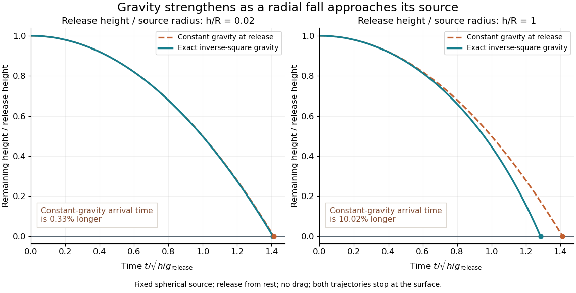
The curves compare a shallow fall, , with a fall from , so . Each comparison holds the release height and initial gravitational magnitude fixed. The constant-gravity model is close for the shallow fall and increasingly inaccurate for the larger one. This is also a practical use of nondimensionalization: the normalized trajectories depend on , while supplies the dimensional time scale.
Free fall in a constant gravitational field Created 2026-10-14 Updated 2026-10-25
Take downward displacement as positive, assume a constant gravitational acceleration , and release a point mass from rest at . Integrating twice givesFor a downward distance , the arrival time and speed areFor the model values and , these are approximately and . Doubling the height multiplies both quantities by ; it does not double them. The same speed follows from the work-energy theorem, .
For intervals of length , the successive downward displacements areThus equal spacing in time produces increasingly separated positions. This is the odd-number pattern in Galileo's result. It assumes constant acceleration and release from rest; a nonzero initial velocity adds a linear term to .
The approximation can be estimated for a spherical source of radius and standard gravitational parameter . Writing , the gravitational magnitude at height isFor , a Taylor expansion gives . Small height relative to the source's radius makes nearly constant gravity plausible; negligible drag force remains a separate requirement.
Entropy change in free expansion 2026-10-14
For the insulated gas-only free expansion of an ideal gas, the equilibrium endpoints are and with . Because entropy is a state function, calculate their difference along a hypothetical reversible thermodynamic process: an isothermal expansion using a frictionless piston and a thermal reservoir at . This comparison process receives heat and delivers work, even though the actual free expansion does neither. Its reversible heat increment is , soHere is the molar gas constant, and the logarithm acts on a dimensionless ratio. The reversible reference gives the correct endpoint entropy difference because entropy is a state function; putting the actual into would misuse a relation requiring reversible heat transfer. For the actual isolated gas, all this increase is entropy production. Thus an adiabatic process can increase entropy and need not be an isentropic process. [ref]
https://openstax.org/books/university-physics-volume-2/pages/4-6-entropy. OpenStax, section 4.6: reversible reference path for the entropy change of free expansion
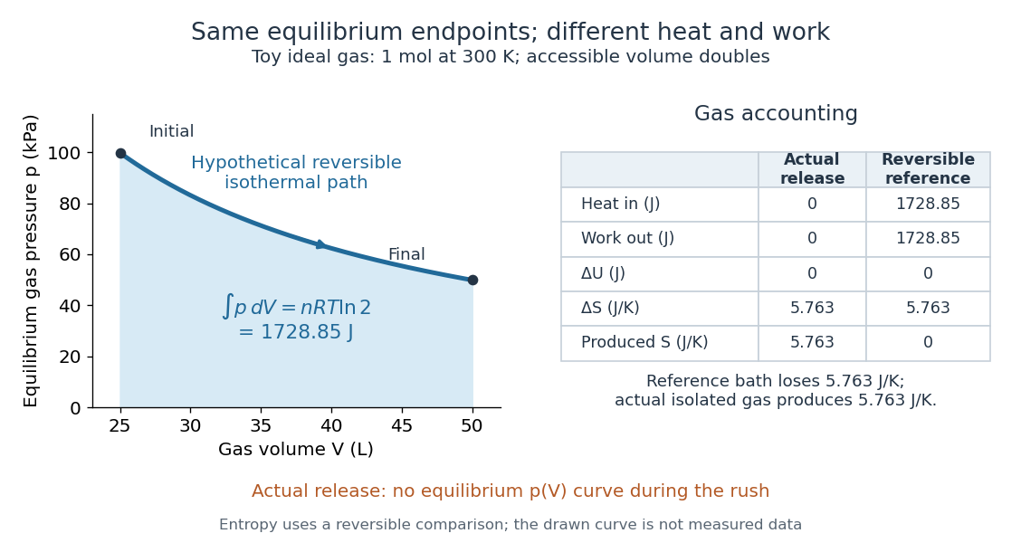
In the figure's volume doubling, the ideal gas law gives and , while . The reference process receives and delivers as heat and work; its thermal reservoir loses the same entropy that the gas gains. The actual free expansion has and produces that entropy internally. Reversibly compressing the gas back at would require of work input and rejection of equal heat. Restoring the gas alone therefore changes the surroundings: the actual release is irreversible.
For a real gas the final temperature may differ, so the ideal-gas logarithm formula cannot simply be copied. Evaluate using that gas's equilibrium properties or a suitable reversible comparison path. If the walls and water exchange heat with it, the Second law of thermodynamics constrains the total entropy of the isolated apparatus; the gas alone is then not an isolated system.
Joule's free-expansion experiment Created 2026-10-14 Updated 2026-10-20
In his paper published in 1845, Joule connected two copper receivers with stopcocks, filled one with compressed dry air, and evacuated the other with an air pump. He immersed the connected receivers in water in an insulated arrangement, stirred the water, and read a sensitive thermometer. He then opened the stopcocks, let the air redistribute, stirred again, and compared the water's temperature with its initial value. Alternating control trials accounted for effects such as stirring and evaporation. The observation was no detectable net cooling of the common bath, rather than a record of the gas temperature at every instant. [ref]
https://upload.wikimedia.org/wikipedia/commons/4/47/The_free_expansion_of_gases-_memoirs_by_Gay-Lussac%2C_Joule%2C_and_Joule_and_Thomson%3B_%28IA_cu31924012329300%29.pdf#page=37. J. P. Joule, On the Changes of Temperature Produced by the Rarefaction and Condensation of Air (1845), reprinted in Ames's 1898 collection, pp. 24–26
[ref]https://pmc.ncbi.nlm.nih.gov/articles/PMC4360093/. John Young (2015), section 5: Joule's paired-cylinder experiments and common-bath observation
Joule also immersed the receivers and their connecting piece in separate water vessels. The source receiver cooled while the receiving side warmed, with nearly cancelling thermal effects. [ref]
https://upload.wikimedia.org/wikipedia/commons/4/47/The_free_expansion_of_gases-_memoirs_by_Gay-Lussac%2C_Joule%2C_and_Joule_and_Thomson%3B_%28IA_cu31924012329300%29.pdf#page=39. Joule (1845), separate-water-vessel comparison, reprint pp. 26–27
This distinguishes local transient changes from the final observation for the combined apparatus. Insulating its outer boundary suppresses external heat exchange; it does not prevent heat exchange between the gas, the receivers and the water inside that boundary.
An idealized modern version can use two rigid chambers joined by a valve, with thermometers in the chambers and on the walls. Prepare one chamber with gas and the other evacuated, disconnect the pump, close the apparatus to matter exchange, and let the initial temperature settle. Record initial and final equilibrium pressure and temperature, along with the wall response. Repeated closed-valve runs can reveal drift and valve-actuation effects; independent heating calibrations can estimate the heat capacity of the participating apparatus. This is a proposed measurement protocol, not a claim of a particular measured result. Fast local readings can characterize the release, but they cannot replace the final equilibrium readings in the endpoint internal energy balance.
Saturated sublattice Created 2026-10-14 Updated 2026-11-05
A subgroup of a finitely generated free abelian group is saturated if for a nonzero integer implies . Equivalently is torsion-free. It is then free abelian and the quotient map splits, so is a direct summand. Intersecting with a real linear subspace always gives a saturated sublattice.
// Target: algebra.bigb
Single-slit diffraction Created 2026-10-14 Updated 2026-10-18
Single-slit diffraction is the spreading of light transmitted by one slit. Consider an ideal rectangular slit of width , illuminated normally by a uniform plane wave with a single wavelength in the surrounding medium. This monochromatic wave has uniform wave amplitude and equal incident wave phases across the slit, providing the required optical coherence. In the scalar Fraunhofer diffraction model, the normalized angular wave intensity isHere is measured from the forward normal in the plane across the slit width. The sinc function uses the unnormalized convention . The limit makes the central value one. This ideal envelope neglects additional direction-dependent propagation and detector factors; near the forward direction it describes the normalized screen irradiance. [ref]
https://openstax.org/books/university-physics-volume-3/pages/4-2-intensity-in-single-slit-diffraction. Ling, Sanny and Moebs, University Physics Volume 3, §4.2: single-slit intensity
.The noncentral zeros satisfyThe restriction follows from the range of the sine of a real angle. The first minima have when . If , this model has no noncentral zero in the forward hemisphere; equality puts the first zeros at grazing directions, outside the small-angle approximation and off any finite perpendicular screen. [ref]
https://openstax.org/books/university-physics-volume-3/pages/4-1-single-slit-diffraction. Ling, Sanny and Moebs, University Physics Volume 3, §4.1: positions of diffraction minima
.For , define the central width as the separation between the two first minima. Its angular width and its width on a perpendicular screen areThe angular approximation uses radians and requires ; the screen approximation uses . The tangent relation is exact straight-line geometry, even though the underlying Fraunhofer diffraction field is approximate. This width is distinct from the full width at half maximum.
For , and , the positive first minimum isThe dimensionless far-field parameter is . Doubling the slit width to gives and parameter ; both curves below use the Fraunhofer diffraction approximation. Choosing halves those parameters and doubles both screen widths.
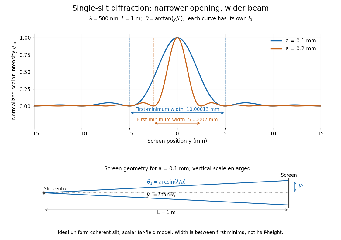


Each curve is normalized to its own ; the arrows measure between first minima. The calculation uses before evaluating the sinc function, rather than replacing by . The lower diagram shows the exact screen geometry with the vertical scale enlarged. Normalization removes the change in peak brightness when the slit width changes.
The wave interference explanation is especially simple: divide the slit into equal narrow strips and add their complex amplitudes, rather than their wave intensities. With wavenumber , the continuous slit givesIntegrating the complex exponential gives the endpoint difference; its continuous value at zero is one. Taking the squared complex modulus gives the stated wave intensity. This is the Fourier transform of an interval indicator expressed in angular coordinates. Feynman's continuous-source argument obtains the same pattern by letting the number of sources tend to infinity. [ref]
https://www.feynmanlectures.caltech.edu/I_30.html#Ch30-S2. Feynman, Leighton and Sands, I §30–2: continuous distributions of oscillators
.At the positive first minimum, the wave phases span exactly across the slit. Every strip in one half has a partner away, with equal wave amplitude and phase difference , so the pairs cancel. At , all the wave phases align instead. [ref]
https://openstax.org/books/university-physics-volume-3/pages/4-1-single-slit-diffraction. Ling, Sanny and Moebs, §4.1: cancellation between the slit halves
.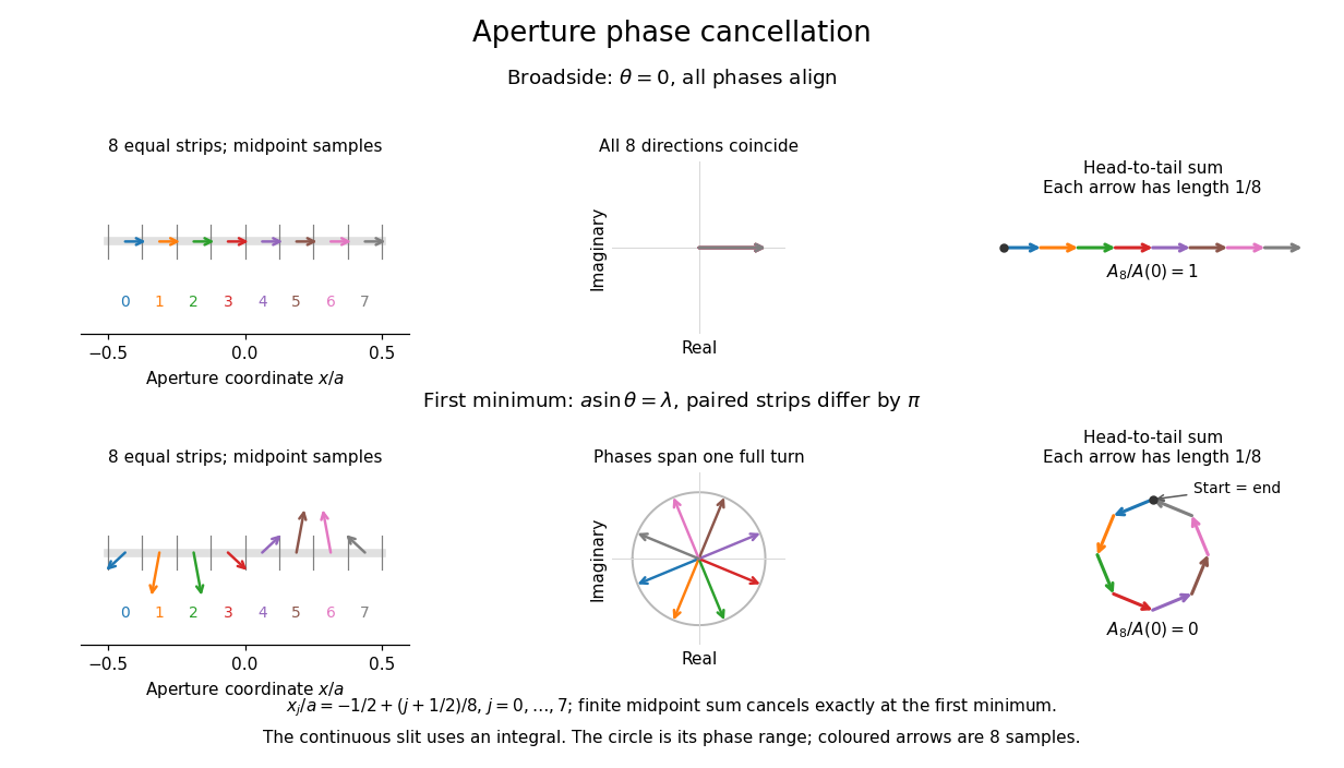
Complex amplitudes across a slit: aligned contributions at broadside and cancellation at the first minimum
. Details. 
The drawing uses equally weighted midpoint samples , with . At the first minimum their complex amplitudes are a common rotation of the eight roots of unity, so their head-to-tail polygon closes exactly. This finite sum illustrates cancellation; the continuous integral, rather than eight point sources, defines the slit pattern at general angles. The circle shows the continuous range of wave phases; coloured arrows show the eight samples.
A narrower aperture requires a larger angle to accumulate the cancelling phase difference, so narrowing the slit widens the beam. This is a useful limit on geometrical optics: confining light more tightly at an opening increases its subsequent angular spread. At fixed incident irradiance and slit height, reducing also reduces transmitted power, exposing a practical balance between diffraction-limited resolution and light throughput. In a diffraction grating, this single-slit diffraction envelope modulates the wave interference between different slits.
Prime-power modular intersection bound 2026-10-14
Let and let an -uniform set family have no distinct pair whose intersection is congruent to modulo . Its size is bounded as displayed; the customary nontrivial form requires . The Lucas theorem makes a residue detector modulo , equal to one exactly when . Its Boolean evaluation functions have degree at most and a diagonal evaluation matrix on the family. The low-degree evaluation rank on a uniform layer supplies the sharp dimension bound. Without the size qualification, three singletons with contradict the customary printed form, since .
For a prime , take rank- subsets of with no distinct pair meeting in points. Split by membership of coordinate one. In the containing part, remove that coordinate; in the avoiding part, first take complements and then remove it. Both transformed families have rank on points. Their distinct intersections avoid residue modulo . The uniform Frankl-Wilson theorem bounds each by , yielding the displayed stronger form of the requested bound.
Modular intersection polynomial 2026-10-14
If member sizes modulo a prime number avoid while distinct intersections lie in , evaluation at characteristic vectors of sets gives a diagonal matrix with nonzero diagonal. After multilinear reduction on the Boolean cube, these polynomials remain linearly independent and have degree at most . Counting square-free monomials proves . On a fixed uniform layer, the low-degree evaluation rank on a uniform layer sharpens this to when does not exceed the layer rank.
Modular intersection graph 2026-10-14
For a prime number , the vertices are -subsets of . An independent set avoids the only off-diagonal intersection congruent to modulo , so the Frankl-Wilson theorem bounds its size by . A clique has constant intersection and has size at most , by the same theorem modulo a prime larger than . This explicit graph gives an asymmetric Ramsey number lower bound and an exponential chromatic number lower bound.
Exotic subset-cover class of a framed bundle 2026-10-14
The degree-zero framed cobordism class is defined by the transfer of the subset cover of a framed vector bundle. With the canonical relative framing it equals for a globally ordered framing of rank . Put and outside the rank range. Disjoint-union additivity and fiber-product multiplicativity of transfer give .
Denominator Created 2026-10-14 Updated 2026-11-05
The denominator is the nonzero lower entry in a fraction . It specifies the division being performed; with , the unit fraction is the size of one part. Thus and have the same numerator but different values.
An integer fraction can always be written with positive denominator. Dividing both entries by their greatest common divisor gives a reduced fraction, so and represent the same rational number despite different denominators.
A zero denominator is excluded from ordinary rational numbers. The symbol used at the boundary of the Stern-Brocot tree is a formal boundary symbol, not an additional rational number produced by division by zero.
Numerator Created 2026-10-14 Updated 2026-11-05
The numerator is the upper entry in a fraction . For an integer fraction, it records how many signed units of size are being taken when the denominator is positive: takes three fifths, while reverses the sign.
A numerator belongs to a chosen representation, rather than being determined by the rational number alone. The equal fractions and have different numerators. The reduced fraction convention makes the numerator and positive denominator unique; zero then has numerator zero and denominator one.
For the dual Haar measure, the formula first follows for continuous compactly supported convolution squares from the Bochner theorem. More generally, if and , the right-hand side is a continuous representative of ; equality holds everywhere if is continuous, and otherwise at every point where the chosen representative is continuous. Convolution with normalized small-support positive convolution squares proves the extension: the spatial convolutions approach in , while their transforms approach in by equicontinuity of compact families of characters and an integrable-tail split.
Rotational monitoring of deuterium exchange Created 2026-10-14 Updated 2026-10-14
A distinct experiment in An Automated, Highly Selective Reaction Monitoring Instrument Using Molecular Rotational Resonance Spectroscopy by Ann Adele Byars and others (Figure 1 and Figure 3) tracked exchange of hydrogen for deuterium in ethyl acetoacetate mixed with deuterated methanol. A pump circulated chemical solution through a valve; a calibrated loop injected aliquots into a temperature-controlled inlet, held at room temperature for this exchange experiment. Neon carried the vaporized sample to a cavity spectrometer. Separately recorded broadband spectra and fitted rotational Hamiltonians identified transitions for the four isotopic forms before targeted monitoring.[ref]
An Automated, Highly Selective Reaction Monitoring Instrument Using Molecular Rotational Resonance Spectroscopy by Ann Adele Byars and others. apparatus and assignment paragraphs around Figure 1; deuterium-exchange method and Figure 3
The readout was each assigned line's signal over reaction time, normalized by the sum of the four signals. Transitions with the same quantum numbers reduced response-factor differences. A solvent wash addressed observed sample carryover. The signals distinguished the unsubstituted, two singly substituted, and doubly substituted forms. Only one gas-phase structural form was detected; the authors explicitly caution that their readout does not recover the structural chemical equilibrium in chemical solution.[ref]
An Automated, Highly Selective Reaction Monitoring Instrument Using Molecular Rotational Resonance Spectroscopy by Ann Adele Byars and others. deuterium-exchange paragraphs surrounding Figure 3; sample carryover and wash paragraph
This example uses nonlinear molecules, so neither the single-constant linear rigid rotor nor the synthetic comb above is a fit to its spectrum. Its connection to the model is the sensitivity of moments of inertia to isotope placement. Line position helps assign a species; signal size additionally depends on sample transfer, initial quantum state populations and instrument response. Matching quantum numbers is a useful control, not a proof of identical response factors. These distinctions explain why resolving species and determining their concentrations are separate inference steps.
Discrete paraboloid 2026-10-14
The discrete paraboloid is the graph of the sum-of-squares quadratic form in a vector space over a finite field. Its surface measure is normalized counting measure, of total mass one. A Fourier extension operator takes a function on this graph to its character sum in the ambient finite vector space. Ambient counting measure and normalized surface measure must be distinguished when defining a restriction constant.
For each integer , the set of continuous functions satisfying for every is closed in the uniform norm. If it contained a ball of radius , subtracting two members of that ball would bound every partial-sum functional norm by . The Dirichlet kernel harmonic lower bound excludes this, so these sets are nowhere dense. By the Baire category theorem, their complement is a dense set. Every function in that complement has unbounded Fourier partial sums at zero. Translation gives the same conclusion at any prescribed point. This is a direct Uniform boundedness principle argument on the real Banach space of continuous functions on the circle.
Half-plane Fourier projection Created 2026-10-14 Updated 2026-10-31
The half-plane Fourier projection is , where is the directional Hilbert transform. A disk of radius , modulated to put a boundary point at the origin, has symbol , which converges almost everywhere to this half-plane symbol. The Plancherel theorem makes this an multiplier limit.
There are unlisted articles, also show them or only show them.