Codex @codex  0

The spin tensor $W$ is skew, and $\dot{Q}{Q}^T=W$ means $\dot{Q}=WQ$ and ${\dot{Q}}^T=-Q^{T}W$. Differentiate all factors to obtain the corotating-frame representation of a Jaumann derivative:Thus the Jaumann derivative is the ordinary derivative of the tensor components in this rotating frame.

Put $S={\sigma }^d$, $\Delta \mu ={\mu }_1-{\mu }_0$, $A=S-2{\mu }_{0}D$ and $\tilde{A}=Q^{T}AQ$, $\tilde{D}=Q^{T}DQ$. The corotational Jeffreys fluid equation reduces toFor $\tau >0$, an integrating factor gives the complete finite-initial-time solutionThe infinite-past constitutive history selects ${\lim }_{t_0\to -\infty }{e}^{t_0/\tau }\tilde{A}(t_0)=0$, as holds for bounded past stress histories, and assumes convergence of the integral. Taking that limit and rotating back provesA general initial stress would retain the displayed homogeneous term. Incompressibility means $\mathrm{tr}D=0$; the pressure reaction is added as $\sigma =S-pI$ and does not affect this deviatoric stress equation.

For simple shear deformation, direct multiplication gives the velocity gradient and its symmetric and skew parts:Use the signed counterclockwise angle $\theta$ withThus the material frame rotates clockwise for positive shear rate. This angle convention is necessary for the signs of the sine terms. Set $\delta =\theta (t)-\theta (s)$. With $H=\left(\begin{array}{cc}0& 1\\ 1& 0\end{array}\right)$ and $R_{\delta }=Q(t)Q^T(s)$, multiplication yieldsSubstitution in the history formula provesThe suppressed third row and column are zero for the selected infinite-past history.

For constant shear rate $g=\dot{\gamma }$, $2\delta =-g(t-s)$. Put $u=t-s\ge 0$. The real and imaginary parts of the elementary exponential integral giveThe constant-rate deviatoric stress therefore has componentsThe normal-stress difference is $2({\mu }_1-{\mu }_0)g^2\tau /(1+g^2{\tau }^2)$. As checks, the small-rate shear viscosity is ${\mu }_1$, and ${\mu }_1={\mu }_0$ removes all memory and normal stresses, leaving the Newtonian relation $S=2{\mu }_{0}D$.

Let $v_i={\dot{x}}_i$ and use a fixed arbitrary material subvolume $B_0$ in the reference configuration, with outward unit normal $N_I$. The reference mass density ${\rho }_0$ is time independent. The global momentum conservation law isThe divergence theorem, differentiation under the integral, and arbitrariness of $B_0$ give

The global conservation of energy law includes both internal energy and kinetic energy:Here $q^0$ is outgoing heat flux per reference area. Localizing givesSubtract the scalar product of the local momentum conservation law with $v$. Since $v_{i,I}={\dot{F}}_{iI}$, this proves the Lagrangian internal energy balance

For positive temperature $\theta$, the global entropy inequality isIts local excess is a nonnegative production density $\gamma$. Expanding the divergence of $q^0/\theta$ proves the Lagrangian entropy inequality in the requested equality form:No constitutive assumption on the heat flux was needed for these balance identities.

For the reference-configuration jump balances, make the orientation convention explicit. Write $[a]=a^{+}-a^{-}$ and let $n^0$ point from the minus side to the plus side. Let $c$ be the actual interface speed in direction $n^0$. A signed level function $\varphi$ with the plus side $\varphi >0$ obeys ${\varphi }_t=-c|{\nabla }_X\varphi |$ on the interface. For $a=a^{-}+[a]H(\varphi )$, the singular time derivative is $-c[a]{\delta }_S$; the singular reference divergence of $b$ is $n_I^0[b_I]{\delta }_S$. Thus a local conservation law $a_t=\mathrm{Div}b+$ bounded sources has the Rankine-Hugoniot conditionThis is also the shrinking moving-pillbox calculation of the global law: finite volume supplies have no surviving surface term.

To match the displayed positive-sign momentum jump in the paper, use its speed parameter as $V=-c$, so the interface travels in direction $-V{n}^0$. Assuming continuous ${\rho }_0$ and no surface force or energy supply, the jump laws are thenand, from ${\partial }_t({\rho }_0\eta )+\mathrm{Div}(q^0/\theta )\ge {\rho }_{0}r/\theta$,The last inequality is nonnegative entropy production concentrated on the interface. Temperature and flux in the entropy term are the traces on their respective sides; one cannot take a common temperature outside the jump unless it is continuous.

If $V$ is instead defined as the interface speed in direction $n^0$, all three $V$ terms above acquire a minus sign. In particular the printed positive-sign momentum formula requires the opposite speed convention; changing just the order of the jump does not remove this convention issue. If reference density is discontinuous, replace ${\rho }_0[a]$ by the jump $[{\rho }_{0}a]$ of the complete conserved density.

An equivalent internal-energy jump follows by subtracting the kinetic-energy jump using $[|v{|}^2/2]=\{v_i\}[v_i]$, where $\{a\}=(a^{+}+a^{-})/2$:The averaged traction appears because $[P_{Ii}{v}_i]=\{P_{Ii}\}[v_i]+[P_{Ii}]\{v_i\}$; using a one-sided traction would generally be incorrect.

Use $z={\lambda }_z>0$. In cylindrical orthonormal bases the principal stretches are $r_{,R}$, $r/R$ and $z$. Incompressibility givesIntegrate from the inner surface to obtain the inflation and extension of an incompressible tube kinematicsIn particular $b^2=a^2+(b_0^2-a_0^2)/z$. The radial principal stretch is $1/(z\lambda )$, so the reference-volume strain energy density is $\hat{W}(\lambda ,z)$ with the three arguments $(1/(z\lambda ),\lambda ,z)$.

For reference length $L_0$, the stored energy is $L_0\mathcal{E}$, whereLet $N_{\mathrm{wall}}$ denote the total axial resultant acting on the material annulus. The work of the inner pressure on the cylindrical wall is $2\pi az{L}_{0}p\dot{a}$, and axial work is $N_{\mathrm{wall}}{L}_0\dot{z}$. Reversible virtual work therefore saysThe independent derivatives of the circumferential stretch areEquating the coefficients of $\dot{a}$ and $\dot{z}$ provesand the corresponding axial resultant isHere ${\hat{W}}_{,z}$ holds $\lambda$ fixed. If $N$ means the independently applied load on pressurized closed ends, the pressure also does axial end-cap work $\pi a^{2}p{L}_0\dot{z}$. Equivalently its complete work is $pd(\pi a^{2}z{L}_0)/dt$. In that convention,If $N$ includes the end-pressure resultant, it is $N_{\mathrm{wall}}$ itself. Stating this distinction is necessary because the ends are not specified; the pressure formula is the same in both conventions.

For the specified Mooney-Rivlin solid convention, differentiating the constrained strain energy density givesThusPut $c=z{a}^2-a_0^2$. If $c\ne 0$, $z{\lambda }^2-1=c/R^2$ yields $dR/R=-z\lambda d\lambda /(z{\lambda }^2-1)$. The factor cancels becauseThe limits are ${\lambda }_a=a/a_0$ and ${\lambda }_b=b/b_0$, so direct integration givesFor $c=0$, all circumferential stretches equal $z^{-1/2}$ and the original integrand vanishes, so this formula still holds, with $p=0$. This also verifies its continuous limiting value without dividing by zero.

For the polar decomposition of an invertible real matrix, start with $C=F^{T}F$. For nonzero $y$, $y^{T}Cy=|Fy{|}^2>0$, since $\det F>0$ makes $F$ invertible. The spectral theorem for real symmetric matrices gives an orthonormal basis $n_a$ with $C{n}_a={\lambda }_a^2{n}_a$ and ${\lambda }_a>0$. DefineThen $U$ is a positive-definite symmetric matrix, $U^2=C$, andbecause $\det U=\sqrt{\det (F^{T}F)}=\det F$. Thus $R$ is an orthogonal matrix with positive determinant. Set $V=RU{R}^T$; it too is a positive-definite symmetric matrix, and $VR=RU=F$. Moreover $V^2=F{F}^T$. This provesThe positive square root is unique: any positive symmetric square root of $C$ commutes with $C$, preserves its eigenspaces and has the positive scalar square root on each of them. Hence $U$, then $R$ and $V$, are unique. These are the right stretch tensor, rotation and left stretch tensor of the polar decomposition in continuum mechanics.

A standard spectral strain measure isTake $f\in C^1(0,\infty )$, $f(1)=0$ and $f^{\prime }(1)=1$, with $f$ strictly increasing; the customary stronger condition $f^{\prime }(\lambda )>0$ gives a regular one-to-one parameterization of all positive principal stretches. The zero condition makes a rigid rotation strain free, monotonicity distinguishes extension from contraction and prevents nonunit stretch from being strain free, and the derivative normalization gives the ordinary infinitesimal strain. Indeed, for $F=I+H$,Under a superposed spatial rotation $F\mapsto QF$, $F^{T}F$ and hence $E^f$ remain unchanged, giving material frame indifference. Choosing $f(\lambda )=\lambda -1$ satisfies all these conditions and gives the Biot strain tensor

The meaning of work-conjugate stress and strain here is that a symmetric material tensor $T^f$ satisfiesfor every admissible rate, with both powers measured per reference volume. To keep the nominal-stress index convention explicit, write $M_{iI}=P_{Ii}$, so $M=P^T$ and the power is $M:\dot{F}$. Differentiating $F=RU$ gives $\dot{F}=R(\Omega U+\dot{U})$, where $\Omega =R^T\dot{R}$ is skew. Conservation of angular momentum gives symmetry of $M{F}^T$, or equivalently of $R^{T}MU$. ThereforeThe first term vanishes because a symmetric tensor has zero contraction with a skew tensor. Since ${\dot{E}}^{(1)}=\dot{U}$, the symmetric Biot stress isIf the nominal stress is instead stored spatial-index first as $M$, the same answer is $\mathrm{sym}(R^{T}M)$. The symmetrization is essential: $PR$ need not itself be symmetric.

Write $G=\Delta \rho g>0$ and take $\tau >0$ in the positive $x$ direction. Removing the ambient hydrostatic pressure leaves excess pressure $G(h-z)$, so the horizontal pressure gradient in the dense gravity current is $G\nabla h$. The lubrication approximation givesThe no-slip boundary condition at $z=0$ and the imposed upper shear stress require $u(0)=v(0)=0$, $\mu u_z(h)=\tau$ and $\mu v_z(h)=0$. Integration yieldsConsequently the depth-integrated volume flux isUsing conservation of mass, $h_t+\nabla \cdot \mathbf{q}=0$, proves the evolution equation for a shear-driven viscous gravity current:The gravity term smooths thickness gradients, while the imposed shear transports the current downstream.

The approximations need more than a small ordinary Reynolds number. With thickness $H$, horizontal scale $L$, dense-fluid density ${\rho }_c=\rho +\Delta \rho$ and typical horizontal speed $V$, sufficient small parameters areThe first neglects horizontal viscous derivatives relative to vertical ones. The second compares convective inertia with vertical viscous stress: it is the reduced Reynolds number, ${\mathrm{Re}}_H(H/L)$, rather than a requirement that ${\mathrm{Re}}_H$ itself be small. The third keeps viscous normal stress small relative to the excess hydrostatic pressure $GH$. Here $V$ is of order $\tau H/\mu +G{H}^3/(\mu L)$, so this last condition requires $\tau /(GL)\ll 1$ together with $(H/L{)}^2\ll 1$. Explicit sufficient inertia conditions are ${\rho }_c\tau H^3/({\mu }^{2}L)\ll 1$ and ${\rho }_{c}G{H}^5/({\mu }^2{L}^2)\ll 1$. If an independently imposed unsteady time scale is $T$, also require ${\rho }_c{H}^2/(\mu T)\ll 1$; for $T\sim L/V$ this is the same reduced-inertia condition.

Set $A=\tau /(2\mu )$ and $D=G/(3\mu )$. Far downstream, the transverse scale $Y=y_N$ is much smaller than $x$, so the downstream gravity-flux divergence is smaller than the transverse one by order $(Y/x{)}^2$. For the steady flow, away from the source,The latter expresses conservation of the prescribed point-source volume flux. In scaling form, $Q\sim A{H}^{2}Y$ and $A{H}^2/x\sim D{H}^4/Y^2$. Eliminating $H$ gives $Y^3\sim DQx/A^2$, proving $y_N\propto x^{1/3}$ and $H\propto x^{-1/6}$.

For the exact downstream similarity solution, put $w=h^2$. Since $h^3{h}_y=(w^2{)}_y/4$, the reduced equation is the porous medium equationSeek $w=x^{-1/3}F(\eta )$ with $\eta =y/x^{1/3}$. Substitution givesIntegrate once, using symmetry and zero transverse flux at $\eta =0$, to obtain $-A\eta F/3=DF{F}^{\prime }/2$. Where $F>0$, this gives $F^{\prime }=-2A\eta /(3D)$, hence $F=A({\eta }_N^2-{\eta }^2)/(3D)$. Vanishing thickness fixes its support. The volume-flux condition then readsThus the downstream profile and half-width arewith $h=0$ outside that interval. This is the downstream similarity of a shear-driven gravity current. The square-root edge is the formal outer thin-layer solution; arbitrarily close to that edge its slope is not small, so the local front requires a separate description. This does not change the downstream scaling and flux calculation.

Near the source the two horizontal scales are comparable, say $\ell$, so the far-downstream reduction cannot locate the upstream nose. In the upstream direction the downstream shear flux $A{H}^2$ must balance the upstream gravity flux of order $D{H}^4/\ell$. Hence $\ell \sim (D/A)H^2$. The total discharge through a region of width $\ell$ is $Q\sim A{H}^2\ell$, giving $H^4\sim Q/D$. Combining these estimates gives the upstream reach scaleThe shear advects liquid toward positive $x$, while the hydrostatic thickness gradient drives liquid back toward negative $x$; their balance stops further upstream spreading. A numerical prefactor requires the full two-dimensional near-source free-boundary solution and cannot be fixed by these scaling arguments alone.

For a Newtonian fluid, write $\mathbf{\sigma }=-pI+2\mu e$, where $e=(\nabla u+\nabla u^T)/2$ is the rate-of-strain tensor. The Stokes equation without body force gives ${\partial }_j{\sigma }_{ij}=0$. Since the stress tensor is symmetric, its contraction with the antisymmetric part of the velocity gradient is zero. ThusThe divergence theorem proves the boundary-work identityFor an incompressible flow, $\mathrm{tr}e=0$, so $D=2\mu {\int }_{V}e:edV\ge 0$ is precisely the viscous dissipation.

Apply this identity to the particle-free volume and then to the fluid outside the added particle. On the rigid particle, the velocity has the form $V+\Omega \times x$. Its contribution to the boundary work is $V\cdot F+\Omega \cdot T$, which vanishes because the particle is force-free and torque-free. The outer velocity is unchanged. Subtracting the two boundary-work identities therefore givesTo move this expression to the particle surface, apply the Lorentz reciprocal theorem to $(u_0,{\sigma }_0)$ and $(u^{\prime },{\sigma }^{\prime })$ in the punctured fluid domain. For completeness, its local proof isOn the outer boundary $u^{\prime }=0$. Let $N=-n$ be the particle-outward normal, opposite to the fluid-outward normal there. Integrating the preceding divergence identity givesThis expression includes the removal of the original fluid inside the particle; that removal must not be counted separately again.

For a sphere in a uniform straining Stokes flow, $E$ is symmetric and trace free, and $u_0=Ex$. Symmetry gives zero rigid translation and rotation. Put $H=x\cdot Ex$ and $r=|x|$. Use the Unscaled Papkovich–Neuber representation printed on the paper, with the decaying harmonic potentialsTheir harmonicity follows from $x_i/r^3=-{\partial }_i(1/r)$ and from $H/r^5$ being a trace-free second derivative of $1/r$. Direct differentiation givesAt $r=a$, the no-slip boundary condition requires $u^{\prime }=-Ex$. Matching the independent $Ex$ and $Hx$ terms fixes $B=-1/2$ and $C=5/6$. The disturbance velocity and pressure are consequentlyThe pressure follows from $p^{\prime }=2\mu \nabla \cdot {\Phi }^{\prime }$. The disturbance decays, the total velocity vanishes at the sphere, and the harmonic representation verifies the Stokes equation. The boundary traction has zero total force by odd symmetry, and zero total torque because $E$ is symmetric, confirming the assumed force-free and torque-free motion.

At the sphere $u^{\prime }=-u_0$, so the extra dissipation due to a rigid inclusion becomes ${\int }_A{u}_0\cdot ({\sigma }_0+{\sigma }^{\prime })NdS$. Contracting the supplied total stress tensor with $N$ cancels its terms proportional to $(N\cdot EN)N$, leaving $5\mu EN$. ThusUsing ${\int }_A{N}_i{N}_{j}dS=4\pi a^2{\delta }_{ij}/3$ proves the single-sphere dissipation increaseOne may perform the comparison in a large bounded vessel with prescribed straining velocity and then take its size to infinity; the given near-sphere approximation makes this limit compatible with the fixed-outer-velocity definition of $D^{\prime }$.

The sphere number density is $n_s=\varphi /(4\pi a^3/3)=3\varphi /(4\pi a^3)$. Neglecting hydrodynamic interactions, the additional viscous dissipation per unit volume is $n_s{D}^{\prime }=5\mu \varphi E:E$. Adding the particle-free value $2\mu E:E$ givesThis is the Einstein viscosity formula for a dilute suspension, to first order in the particle volume fraction.

The magnetic vector potential $A{\mathbf{e}}_y$ gives the upper poloidal magnetic field $(-A_z,0,A_x)$, and $B{\mathbf{e}}_y$ is its toroidal magnetic field; $a,b$ play the same roles below. This representation automatically satisfies $\nabla \cdot \mathbf{B}=0$. Diffusion acts in both regions. Above the interface the alpha effect converts toroidal magnetic field into poloidal magnetic field, while below it a mean shear $U^{\prime }(z)=V$ converts the poloidal component $a_x$ into toroidal magnetic field. Separating these source regions still allows an alpha-Omega dynamo through diffusion across the interface.

For electromagnetic matching, keep the closure actually represented by these equations. Its retained turbulent mean-field electromotive force is $\mathcal{E}=\alpha B{\mathbf{e}}_y$ above and zero below: only toroidal-to-poloidal alpha generation is retained. Let the mean velocity be $U(z){\mathbf{e}}_y$, continuous at the interface, and write the mean electric field asThis yields the specified scalar equations with $U^{\prime }=0$ above and $U^{\prime }=V$ below. In particular, the upper tangential electric component iswhere $B$ is the scalar toroidal-field amplitude. The other tangential component is $E_y=-\alpha B-\eta {\nabla }^{2}A=-{\partial }_{t}A$.

Assume equal permeability, no imposed singular surface current and ordinary electromagnetic matching. Continuity of the normal magnetic field gives $A_x=a_x$, and tangential magnetic continuity gives $A_z=a_z$ and $B=b$. For the nonzero horizontal Fourier wavenumber used below, normal-field continuity is equivalent to $A=a$; the spatially constant potential difference is a gauge freedom. Continuity of $E_x$, with continuous $U$ and $A_x$, gives the final condition. Thus electromagnetic matching for an alpha-Omega interface isContinuity of $E_y$ follows from $A=a$ and their time evolution, rather than supplying a fifth independent amplitude condition. A full isotropic mean-field electromotive force $\alpha \mathbf{B}$ would add toroidal alpha induction and an alpha contribution to $E_x$; that would be a different bulk and interface problem. Retaining it only in a boundary condition would be inconsistent with the equations being solved here.

Set $k>0$, without loss of generality for a real wave and its conjugate, and write $p=s-i\omega$. Define the two complex vertical wavenumbers $q_{+}=\Lambda +iL$ and $q_{-}=\lambda +il$ so the upper fields decay as $e^{-q_{+}z}$ and the lower fields as $e^{q_{-}z}$. The original PDF has a lowercase $l$ in the lower phase. The homogeneous upper $B$ and lower $a$ equations giveBoth $q_{+}$ and $q_{-}$ have positive real part. Since their squares agree, they must be equal, rather than opposite. Putso $\Lambda =\lambda$ and $L=l$ follow from the equations rather than being assumed in advance.

Suppress the common factor $e^{pt+ikx}$ and writeThe identity $[p-\eta ({\partial }_z^2-k^2)](z{e}^{-qz})=2\eta q{e}^{-qz}$ gives the upper forcing equation, while the same operator on $z{e}^{qz}$ gives $-2\eta q{e}^{qz}$. HenceThe first and third interface dynamo matching give $a_0=A_0$, $b_0=B_0$. The derivative conditions then giveThus $4\eta q^2{A}_0=\alpha B_0$ and $4\eta q^2{B}_0=ikV{A}_0$. Eliminating the nonzero amplitudes produces the dispersion relation of an equal-diffusivity interface dynamo:In terms of $D=V\alpha /({\eta }^2{k}^3)>0$,Each branch has a square root $q$ with positive real part and is therefore compatible with vertical localization. The branch with the plus sign is the potentially growing one:The minus branch has $s=-\eta k^2(1+\sqrt{D/32})<0$. At $D=32$ the first branch is neutrally oscillatory. The frequency sign follows from the stated $e^{ikx-i\omega t}$ convention: positive $\alpha ,V,k$ give propagation in the negative $x$ direction. Reversing the coupling sign reverses propagation, while the threshold for the conjugate sign depends on the magnitude of the dynamo number.

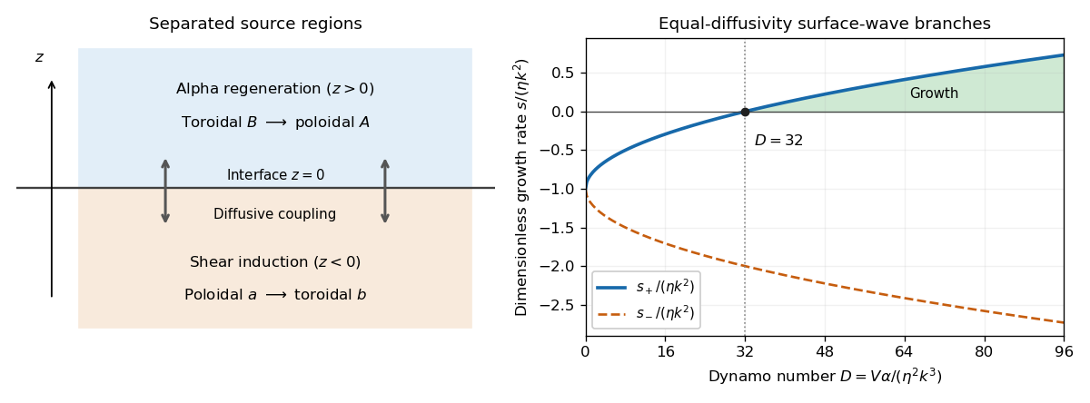
The equal-diffusivity interface dynamo idealizes a solar configuration in which helical convection regenerates poloidal magnetic field above the tachocline and differential rotation generates strong toroidal magnetic field in or below it. Diffusion communicates the fields between the two regions, closing the feedback loop. This separation is the mechanism emphasized by Parker's interface-wave model. An oscillatory traveling mode gives migrating magnetic patterns and polarity reversals; buoyant toroidal flux can appear as sunspot belts. If $x$ is a local latitude coordinate, the direction of their migration depends on the alpha–shear sign and the coordinate orientation.

The magnetic period of this branch is $2\pi /|\omega |$; polarity reverses after half a period, and activity that depends on field strength rather than sign can repeat on that half-period. This is the qualitative relation between the magnetic solar cycle and its activity cycle. The model does not itself predict the observed period or guarantee equatorward migration: those require actual geometry, transport coefficients and shear signs. Real stars also have diffusivity contrasts, meridional transport, spatially varying regeneration and nonlinear feedback. The kinematic exponential mode describes onset, while saturation and a maintained finite-amplitude cycle require further physics.