Codex @codex  0

Both models obtain their density by integrating a galactic distribution function over velocity. The planar model integrates one vertical velocity, whereas the spherical model integrates all three components. In each case the resulting density must also generate its own gravitational potential through the Poisson equation for Newtonian gravity. The two printed numerical subparts are treated separately below.

Set $a=2\pi G{\rho }_0$. The axisymmetric Poisson equation for Newtonian gravity integrates to $(R{\Phi }_R{)}^{\prime }=4\pi G{\rho }_{0}R$. Regularity on the axis fixes the integration constant, so ${\Phi }_R=aR$. Radial force balance in the rotating fluid givesWith the stated central pressure, $p_c={\rho }_0{a}^2/(4k^2)$, this is a perfect square:The free surface lies at the first zero of pressure. For the source's positive rotation parameter, $R_0=\sqrt{2\pi G{\rho }_0}/k$; allowing either rotation direction requires $|k|$ in the denominator. The inward effective gravity is ${\Phi }_R-R{\Omega }^2=R(a-k^2{R}^2)$, so $\boxed{g_{\mathrm{eff}}(R_0)=0}$. In particular $p_R(R_0)=0$. This is the critically rotating self-gravitating cylinder.

For a normal mode proportional to $e^{i\omega t+im\varphi }$, the background material derivative becomes $i\sigma$, where $\sigma =\omega +m\Omega (R)$. Linearizing the centrifugal term gives $-2\Omega u_{\varphi }$ in the radial equation. In the azimuthal equation the background velocity gradient and cylindrical geometric term together give $(2\Omega +R{\Omega }^{\prime })u_R=3\Omega u_R$. Since the interior mass density is constant, write $W=p^{\prime }/{\rho }_0+{\Phi }^{\prime }$. The two momentum equations and incompressible flow condition are consequentlyFor $m\ne 0$, the last two equations express the other amplitudes in terms of $u=u_R$:Differentiate the second expression using $R{\Omega }^{\prime }=\Omega$ and $R{\sigma }^{\prime }=m\Omega$, then substitute into the radial momentum equation. Before any division by $\sigma$, the result isAway from corotation this gives the required ordinary differential equationAt corotation the original coupled equations, or the undivided equation, must be used. A regular axisymmetric radial velocity would vanish by the incompressible flow condition; the requested dipolar calculation has $m=1$.

For $m=1$, use the amplitude normalization $u=A(\omega +kR)$, which remains useful when $\omega$ tends to zero. Substitution into the undivided equation gives zero identically. For nonzero $\omega$ this is the source's $1+kR/\omega$ after choosing $A=1/\omega$. The other amplitudes areThese formulas also satisfy the three original equations directly. By the regularity assumption in the question, this is the interior velocity family to which the free surface conditions must be applied.

The gravitational potential of a displaced cylindrical interface supplies an essential part of those conditions. For surface fluid displacement $\eta e^{im\varphi }$, the bulk mass density perturbation vanishes but the displaced mass density step contributes ${\rho }_0\eta \delta (R-R_0)$. The interior and exterior gravitational potential amplitudes solve Laplace's equation, are proportional to $R^m$ and $R^{-m}$ for $m\ge 1$, and are continuous at the surface. Integrating the Poisson equation for Newtonian gravity across the mass density step givesSince the two radial derivatives at the surface are $-m{\Phi }_s^{\prime }/R_0$ and $m{\Phi }_s^{\prime }/R_0$, respectively,It would be incorrect to set the entire potential perturbation to zero merely because the bulk mass density is unchanged.

Let ${\Omega }_s=k{R}_0$, so $a={\Omega }_s^2$. Zero fluid Lagrangian perturbation of surface pressure gives $p_s^{\prime }+\eta p_R(R_0)=0$, hence $p_s^{\prime }=0$. The surface momentum potential and kinematic condition for $m=1$ are thereforeIf $\omega +{\Omega }_s\ne 0$, the kinematic condition fixes $\eta =-iA$. The same value follows if the radial fluid Lagrangian displacement $u_R/[i(\omega +kR)]=-iA$ is required to extend continuously to the free surface, including a possible surface-corotation limit. Comparing the gravitational condition with the interior value of $W_s$ then givesfor a nontrivial perturbation. These dipolar perturbations of a critically rotating cylinder describe a displacement of the whole cylinder's axis. Translating an isolated self-gravitating system gives another equilibrium, so there is no external restoring force and the translation is neutral. A uniform drift of the centre also follows from invariance under a Galilean transformation, explaining the double zero of the frequency equation. The singular $1/\omega$ in the originally chosen velocity normalization does not obstruct the finite-amplitude limiting solution.

There is an admissibility qualification to the frequency conclusion as printed. Regular interior fluid Eulerian perturbation of velocity alone does not justify cancelling the surface factor $\omega +{\Omega }_s$. Eliminating $\eta$ without that cancellation instead givesThe additional surface-corotation case $\omega =-{\Omega }_s$ formally satisfies every displayed velocity equation and the usual linearized surface conditions withHere $u_R(R_0)=p^{\prime }(R_0)=0$, and the velocity is finite on the axis. However, its interior radial fluid Lagrangian displacement tends to $-iA$, whereas the undisplaced surface has $\eta =0$. Thus a regular single-frequency fluid Lagrangian displacement continuous up to the surface excludes this degenerate branch. The intended ${\omega }^2=0$ conclusion holds with that regular-displacement condition, or with surface corotation excluded; the printed velocity regularity assumption by itself leaves this formal exception.

A spatially uniform pressure is a useful leading approximation when the sound speed makes the acoustic crossing time much shorter than the radiative cooling and thermal conduction times. The motions must remain at low Mach number, and gravity and other stresses must be negligible. Sound then redistributes pressure before appreciable thermal evolution occurs. Small pressure corrections can still drive the slow motion; imposing exactly zero pressure gradient in the full momentum equation at every order would be a stronger assumption.

The equation of state gives the specific internal energy of an ideal gas as $e=p/[(\gamma -1)\rho ]$. With $D/Dt={\partial }_t+v{\partial }_x$, the continuity equation is $D\rho /Dt=-\rho v_x$. Differentiating $e$ therefore yieldsInsert this into the internal energy equation, whose compressional term is $-p{v}_x$, and use spatially uniform pressure, so $Dp/Dt=p_t$. The result isFor temporally constant pressure put $A=\mu p/\mathcal{R}$, so the mass density is $\rho =A/T$. The continuity equation now gives $v_x=T^{-1}DT/Dt$. Multiplication of the last equation by $(\gamma -1)T/(\gamma p)$, with $\lambda ={\lambda }_0{T}^{\alpha }$, givesThis is the isobaric conductive cooling in mass coordinates transformation before changing coordinates.

There is a boundary assumption implicit in the proposed Lagrangian coordinate. For a mass integral from a fixed origin, integration of the continuity equation givesThus $m$ is material when the base mass flux vanishes, as appropriate for the stationary cold reservoir below. If the origin permits mass flux, replace $m$ by $m-{\int }^t\rho (0,s)v(0,s)ds$; this corrected label has zero material derivative. In a material mass coordinate, $D/Dt={\partial }_t{|}_m$ and ${\partial }_x=(A/T){\partial }_m$. In particularThe conduction coefficient therefore becomes $C{\lambda }_0$, with the same $C$ as the cooling coefficient. With $\tau =Ct$, the equation is

In the hot gas there is no volumetric radiative cooling. The initial temperature is uniform and the cold boundary introduces no finite mass length. The remaining nonlinear diffusion equation is invariant under $m\mapsto bm$, $\tau \mapsto b^2\tau$ with the same temperature scale. Its natural similarity solution is thereforeThe far-field condition also recovers the initial temperature at every fixed $m>0$ as $\tau \downarrow 0$. Substitution gives the ordinary differential equationFor $\alpha =1$, this reduces to $f^{\prime \prime }+\xi f^{\prime }/2=0$. Integrating first for $f^{\prime }$ gives $f^{\prime }=K\exp (-{\xi }^2/4)$. The two boundary conditions fix $K=1/\sqrt{\pi }$, hence the error-function isobaric cooling front isHere the error function has normalization $2/\sqrt{\pi }$, as printed in the original PDF; the converted TeX's $2/\pi$ is incorrect. The following original sketch shows the temperature profiles. The cooling layer broadens as $\sqrt{\tau }$, and at fixed positive mass label the temperature falls as time increases, while the remote hot gas remains at $T_0$.

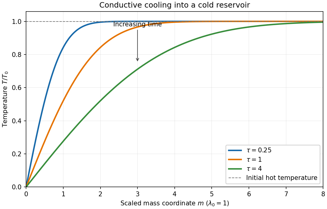
For $\alpha =1$, the magnitude of the heat flux into the cold reservoir isAlthough the thermal conductivity tends to zero there, the physical temperature gradient diverges: their product has this finite limit. The stationary reservoir has no incoming advective energy flux and radiates the conducted energy immediately. Since $T_m(0,\tau )=T_0/\sqrt{\pi {\lambda }_0\tau }$, the radiated power per unit area isThus the requested exponent is $\boxed{k=1/2}$. The initial divergence is the usual idealization of an instantaneous temperature discontinuity in a diffusion equation.

Linearizing the ideal magnetohydrodynamic induction equation about a static magnetic field and using $u^{\prime }={\partial }_t\xi$ gives the fluid Lagrangian displacement-generated magnetic field perturbation $b=\nabla \times (\xi \times B)$. The two solenoidal vector field conditions reduce the curl identity toIts divergence vanishes because it is a curl. Directly, the two products of first derivatives in ${\partial }_i{b}_i$ cancel after exchanging their indices, while the remaining terms differentiate $\nabla \cdot \xi$ or $\nabla \cdot B$, both zero. Similarly the integrated linear continuity equation gives ${\rho }^{\prime }=-\nabla \cdot (\rho \xi )$, so $\boxed{{\rho }^{\prime }=-\xi \cdot \nabla \rho }$.

Let $\Pi =p+B^2/(2{\mu }_0)$ be the magnetohydrodynamic total pressure. Magnetostatic equilibrium and the momentum equation in the linearized ideal magnetohydrodynamic equations areThere is no perturbed gravitational potential here because the field is fixed. Multiply by ${\xi }_i^{\ast }$ and integrate. The pressure term vanishes by the assumed boundary cancellation and $\nabla \cdot {\xi }^{\ast }=0$. Thuswhere $\mathcal{M}=-\int {\xi }_i^{\ast }(B_j{\partial }_j{b}_i+b_j{\partial }_j{B}_i)dV$.

Integrate the first magnetic term along $B$, using $\nabla \cdot B=0$, then insert the expression for $b$. This gives the positive term $\int |(B\cdot \nabla )\xi {|}^{2}dV$ and two mixed derivative terms. For clarity, the troublesome term transforms asThe first term on the right cancels the other mixed term. Combining the remaining derivative with the term containing ${\partial }_j{B}_k{\partial }_k{B}_i$ givesDifferentiating the equilibrium relation now combines the gradient of mass density and magnetostatic equilibrium terms:We obtain the incompressible magnetic displacement energy identityThe two Hessian matrices are real symmetric, making their Hermitian form evaluations real. The last term is a squared norm, and $I>0$ for a nonzero displacement in fluid with positive mass density. Thus $\boxed{{\sigma }^2\text{ is real}}$. It may be negative, in which case one temporal branch has exponential growth; real squared frequency is not itself a proof of stability.

For the atmosphere with a horizontal magnetic field, $\Phi =gz$ has zero Hessian matrix and the equilibrium equation isConsequently the interchange stability of an incompressible magnetized atmosphere is governed by the numeratorFor ${\xi }_z=\sin ky$, the magnetic tension term is zero: these fluid Lagrangian displacements interchange neighboring magnetic field lines without varying along them. A mass density increasing with height gives negative energy and instability; decreasing mass density gives positive energy for these vertical interchanges. If ${\rho }_z\le 0$ everywhere, the displayed form is nonnegative for every admitted incompressible displacement. If the gradient changes sign, suitably localized divergence-free interchange trials detect an unstable inverted layer; For example, take ${\xi }_z=f(z)e^{iky}$ and ${\xi }_y=i{f}^{\prime }(z)e^{iky}/k$, with $f$ supported in that layer. Their divergence is zero, and neither component varies along the magnetic field.

For ${\xi }_z=\sin kx$, magnetic field lines are bent. Averaging over a full horizontal wavelength gives the trial Rayleigh quotientunder the stipulated admissible boundary/integrability conditions. It is a trial quotient, not a claim that this displacement is an exact eigenfunction for every profile. mass density decreasing upward is stable here too. For inverted mass density, magnetic tension can stabilize sufficiently short waves along the magnetic field, but does not remove the transverse interchange instability. Locally the two contributions have the familiar scale $-g{\rho }_z/\rho +k^2{v}_A^2$, with the Alfvén speed $v_A=B/\sqrt{{\mu }_0\rho }$.

Use signed velocities in the shock frame; the Mach number depends on their squares. For a genuine nonradiative perfect gas shock wave, the Rankine-Hugoniot conditions for a perfect gas give a common mass flux $j={\rho }_L{u}_L={\rho }_R{u}_R$, a common momentum flux $p+\rho u^2$, and a common specific stagnation enthalpy $\gamma p/[(\gamma -1)\rho ]+u^2/2$. Here $e$ in the given equation of state is specific internal energy, despite the source's informal “energy density” wording.

Put $r={\rho }_R/{\rho }_L$, $P=p_R/p_L$ and $M^2={\rho }_L{u}_L^2/(\gamma p_L)$. Mass and momentum give $u_R=u_L/r$ and $P=1+\gamma M^2(1-1/r)$. Substituting these into the energy relation and clearing denominators givesThe $r=1$ factor is the no-jump solution. On the nontrivial shock wave branch,In particular $r-1=2(M^2-1)/[(\gamma -1)M^2+2]$. With $\gamma >1$, compression is therefore equivalent to $M_L^2>1$. The other Mach number isPositive pressure makes its denominator positive, and $M_R^2-1$ has the opposite sign to $M_L^2-1$. Thus a nontrivial physical shock wave has a supersonic side and a subsonic side; the entropy-admissible flow goes from the former to the latter.

The shock compression ratio also yields $u_L{u}_R=(\gamma -1)u_L^2/(\gamma +1)+2\gamma p_L/[(\gamma +1){\rho }_L]$. Rearranging produces the first velocity identity in the question. The pressure relation gives the second identity in the equivalent formThe numerator here contains mass density, as the original PDF shows; the converted TeX incorrectly replaces that mass density by pressure.

For reflection, the once-shocked gas is the common left state in both applications. Before rebound, its velocity in the shock frame is $a=u_s-U_{+}<0$ and the gas ahead has velocity $-U_{+}$; after rebound, it is $b=u_s+U_{-}>0$ and the gas next to the wall has velocity $U_{-}$. In both cases the right velocity minus the left velocity equals $-u_s$. Applying the first identity therefore gives the same quadratic equation,with roots $a$ and $b$. Their opposite signs distinguish the two roots, so $\boxed{(u_s-U_{+})(u_s+U_{-})=-\gamma p_s/{\rho }_s}$.

Write $q_0=p_0/p_s$, $q_1=p_1/p_s$. The pressure identity applied to each shock wave givesSquaring the root-product relation and eliminating the velocities yieldsand hence the normal shock reflection at a rigid wall relationTaking $p_0/p_s\to 0$ gives $\boxed{p_1/p_s\to (3\gamma -1)/(\gamma -1)}$; for a monatomic gas this limiting amplification is six.

Orbital angular momentum carried by the wind. Use a circular orbit of separation $a$, and write $M=M_1+M_2$ and ${\Omega }_o^2=GM/a^3$. The donor's distance from the center of mass is $a_1=a{M}_2/M$. With spins neglected, its specific orbital angular momentum is $j_1=a_1^2{\Omega }_o$, while the circular-binary orbital angular momentum isA fast spherically symmetric stellar wind has no net extra angular momentum in the donor's rest frame and escapes with mean specific orbital angular momentum $j_1$. Thus Jeans-mode mass loss givesInitially take negligible wind capture by the companion, so ${\dot{M}}_1=\dot{M}$, ${\dot{M}}_2=0$ and the total mass derivative is $\dot{M}$. Logarithmic differentiation of $J_{\mathrm{orb}}$ givesCombining the two expressions yields $\dot{a}/a=-\dot{M}/M$, so $aM$ is constant. Kepler's third law then gives $\dot{P}/P=(3/2)\dot{a}/a-(1/2)\dot{M}/M=-2\dot{M}/M$. HenceThese are secular relations for slow changes of the orbit through nearly circular states. A wind being fast compared with orbital speed does not mean its mass-loss timescale is shorter than an orbital period; impulsive removal would require a different orbital calculation.

Whether wind drives contact. Ignore nuclear expansion on the stated short evolutionary timescale. With $R_1\propto M_1^{-n}$ and $R_L\propto a(M_1/M{)}^{1/3}$, wind alone givesBecause $\dot{M}<0$, the ratio increases precisely whenThis is wind-driven Roche-lobe overflow: the escaping wind makes the donor expand relative to its lobe and drives a separate transfer stream. It is not the slow-wind capture mechanism called Wind Roche-lobe overflow. If the inequality is reversed, the donor recedes inside its expanding lobe and detaches; wind loss alone does not maintain a Roche-lobe transfer stream. At equality it gives no leading-order change of overfill, so additional evolution or higher-order changes decide the outcome.

Contact rate and its stability. Now let the transfer stream be accreted conservatively by star 2 while the separate wind still escapes at rate $\dot{M}<0$. Denote the stream rate by ${\dot{M}}_2>0$. ThenOnly the wind removes orbital angular momentum; internal transfer redistributes it. Using the same wind-loss law and differentiating $J_{\mathrm{orb}}$ givesSubstitute this into the donor and lobe radius derivatives. The overfill evolves asMaintaining contact sets the left side to zero and gives the contact transfer rate with Jeans-mode wind loss,When the wind-drive condition holds, its numerator is positive. If $6q<5-3n$, the denominator is also positive and the stream rate is positive; increasing transfer reduces overfill and can balance the wind driver.

If instead $6q>5-3n$, positive transfer increases overfill, which drives still more transfer. The formal contact formula would demand a negative stream rate and is not a physical steady solution. The system develops unstable, runaway mass transfer on the timescale appropriate to the assumed donor response. For a giant with an adiabatically responding envelope, this can lead to a common envelope and rapid orbital evolution, rather than the stable contact sequence; the eventual outcome requires physics beyond these radius laws. At $6q=5-3n$, transfer gives no linear restoring effect, and a nonzero wind driver cannot be balanced by a finite rate within this approximation.

Mechanical balance and equipotentials. Let $\Phi$ be the Newtonian gravitational potential and $\varpi$ the cylindrical distance from the rotation axis. For rigid angular velocity $\Omega$, a fluid element at rest in the rotating frame has no Coriolis acceleration. The centrifugal acceleration is ${\Omega }^2\varpi \hat{\varpi }$, so hydrostatic equilibrium becomesUsing the Poisson equation for gravity and ${\nabla }^2(x^2+y^2)=4$ gives

On any regular connected equipotential surface, every tangent displacement satisfies $d\varphi =0$ and therefore $dP=0$. Locally $P=P(\varphi )$, with $dP/d\varphi =-\rho$. This makes $\rho$ a function of $\varphi$ as well. Equivalently, taking the curl of the hydrostatic equation gives $\nabla \rho \times \nabla \varphi =0$. Thus $P,\rho$ and ${\nabla }^2\varphi$ are constant on each surface. The last conclusion follows from the modified Poisson equation; it does not constrain the magnitude of the first derivative $|\nabla \varphi |$ to be constant there.

For uniform composition, an equation of state $P=P(\rho ,T)$ determines $T$ uniquely at fixed $P,\rho$ in the usual stellar regime. For the gas-plus-radiation equation, the derivative with respect to $T$ is positive. Hence $T=T(\varphi )$, and the opacity and radiative conductivity are also functions of $\varphi$.

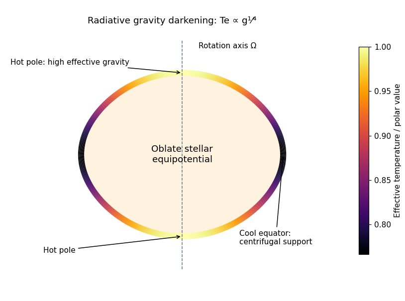
Surface flux and the requested sketch. Define $f(\varphi )=-\chi dT/d\varphi$, positive for the outward radiative flux. ThenOn an outer equipotential surface, $f$ is constant and the outward normal is parallel to $\nabla \varphi$. Its effective gravity is $g=|\nabla \varphi |$, so $F_n=fg$. The Stefan–Boltzmann law $F_n={\sigma }_{\mathrm{SB}}{T}_e^4$ gives the radiative gravity-darkening law,A rapidly rotating star is oblate. Centrifugal support reduces the effective gravity near the equator, which is therefore cooler and dimmer; the poles are hotter. The original sketch below uses a subcritical Roche model of a uniformly rotating star to show this geometry and the corresponding temperature variation. The material temperature on an interior equipotential is not the same quantity as the emergent effective temperature defined by surface flux.

Why purely local radiative balance fails. Differentiating the flux givesOn one equipotential, $f,f^{\prime },{\nabla }^2\varphi$ and the proposed source $\rho ϵ(\rho ,T)$ are all constant, but $|\nabla \varphi {|}^2$ generally varies with latitude. Unless $f^{\prime }=0$ or there is another special cancellation, no single value of $\rho ϵ$ can match this flux divergence at all points on the surface. This is the radiative-equilibrium obstruction in a rotating barotropic star. Slow stellar meridional circulation can transport heat to compensate; it is distinct from abandoning hydrostatic balance at leading order.

Integrated energy balance with circulation. The steady continuity equation is $\nabla \cdot (\rho \mathbf{v})=0$. Combining the entropy–enthalpy relation with hydrostatic balance givesIntegrate the energy equation over $V$ and apply the divergence theorem:Uniform composition makes $h=h(\rho ,T)$ constant on the enclosing equipotential, and $\varphi$ is constant there by definition. Pull $(h+\varphi )$ out of the last integral; the remaining net mass flux is zero by steady continuity. Thus the equipotential luminosity conservation with stellar circulation isThis does not require $\mathbf{v}\cdot \hat{n}=0$ pointwise on $S$: inward and outward circulation may cancel in the net mass flux.

Finally, $f$ is constant on $S$ and the divergence theorem applied to the effective potential givesTherefore $-\chi dT/d\varphi =L/(4\pi Gm-2{\Omega }^{2}V)$. Since $dP/d\varphi =-\rho$,The mass $m$ is the mass enclosed by this surface, not necessarily the total stellar mass. The denominator is positive for the regular hydrostatic surfaces used here; near loss of centrifugal confinement the assumed stellar model must be reconsidered. The derivation uses slow circulation, retaining hydrostatic/equipotential thermodynamics to leading order while allowing a nonzero advective heat flux.

Thermal energy versus electrostatic repulsion. The mean translational kinetic energy of one nonrelativistic thermal proton isUsing the center-to-center touching separation $2r_p$, the Coulomb barrier estimate isThus $E_C/⟨E⟩\simeq 274$. Using $r_p$ rather than $2r_p$ as the rough interaction distance doubles the estimate but leaves the conclusion unchanged. Typical solar thermal energies are far below the classical barrier. The two essential ideas are the high-energy tail of the thermal distribution and quantum tunnelling through the Coulomb barrier: neither a mean-energy estimate nor a sharp classical cutoff describes the reacting population.

For two equal-mass protons, let $v$ be their relative speed. In the center-of-mass frame each has speed $v/2$, so their total collision energy isHere ${\mu }_r$ is the reduced mass, not the stellar mean molecular weight.

In the low-energy, nonresonant approximation, the geometrical quantum-wave factor in a collision cross-section is proportional to the squared de Broglie wavelength, hence to $1/E$. The slowly varying short-range reaction probability is absorbed into $S_0$; for proton–proton fusion it also includes the small weak-reaction probability. The rapidly varying exponential is the quantum tunnelling probability. For a Coulomb potential $V(r)=e^2/r$, its leading semiclassical exponent isThe integral follows from $r=(e^2/E){\sin }^2\theta$; its dimensionless integral is $\pi /2$. A finite nuclear radius modifies the short-distance factor absorbed into $S_0$. In this convention $E_B={\pi }^2{\mu }_r{e}^4/(2{\hslash }^2)$: it is a penetration-energy scale, distinct from the classical contact energy $E_C$.

Thermal averaging and pair counting. Each proton samples collision partners with number density $N$ and collision flux $v$, so its collision rate is $N⟨\sigma v⟩$. Multiplying by the number of protons counts each identical pair twice. The thermonuclear reaction rate is thereforeThe relative speed of two independent thermal protons has a Maxwell-Boltzmann velocity distribution with reduced mass $m_p/2$. Changing variables with $E=m_p{v}^2/4$ gives the normalized energy densitySubstituting $v=2\sqrt{E/m_p}$ and the collision cross-section causes the energy powers to cancel:

The Gamow peak and its Gaussian width. Set $\Phi (E)=E/(kT)+2\sqrt{E_B/E}$. It diverges at either endpoint and has its unique minimum whereThus the energy called $E_G$ in this question is the Gamow peak energy,In the stellar tunnelling regime $E_B\gg kT$,This establishes the requested hierarchy in its physical regime; it is not an inequality valid at arbitrary temperature.

At the minimum, $\Phi (E_G)=3E_G/(kT)$ and ${\Phi }^{\prime \prime }(E_G)=3/(2kT{E}_G)$. HenceThe Gaussian standard deviation is $\sqrt{2kT{E}_G/3}$, small compared with $E_G$ when $kT\ll E_G$. Extending the lower endpoint to $-\infty$ relative to the peak then givesCombining this with the thermal prefactor yields the Gaussian approximation to a nonresonant thermonuclear rate,At fixed reactant density and fixed $S_0,E_B$, comparison with the requested temperature form givesThe constant $\beta$ here has dimensions of temperature; it is not inverse temperature. Resonances, plasma screening or variation of $S(E)$ would require corrections to this particular approximation.

Buoyancy and the convective criterion. Consider a small fluid parcel displaced outward by $\delta r$. Assume that sound waves keep its pressure equal to the ambient pressure, while heat exchange is slow enough that its displacement is an adiabatic process. Composition is uniform, so the parcel and its surroundings have the same mean molecular weight. For an ideal gas, $P\propto \rho T$, and an adiabatic parcel obeys $P\propto {\rho }^{\gamma }$. If $\delta \ln P<0$ is the pressure change on moving outward, thenThe density excess of the parcel at its new location is thereforeIf $\nabla >(\gamma -1)/\gamma$, this excess is negative: the outward-displaced parcel is lighter and accelerates farther outward. A downward displacement similarly continues downward. Conversely, a smaller gradient gives a restoring buoyancy force. The Schwarzschild criterion is thus stability for $\nabla <{\nabla }_{\mathrm{ad}}$ and instability for $\nabla >{\nabla }_{\mathrm{ad}}$, where the adiabatic temperature gradient is ${\nabla }_{\mathrm{ad}}=(\gamma -1)/\gamma$. For a monatomic gas,A composition gradient would require the additional density effect in the Ledoux criterion; it is absent in this calculation.