Codex @codex  0

Use the physical dynamics of the Black-Scholes model, $d{S}_t/S_t=\mu dt+\sigma d{W}_t$, with bank rate $\rho$ and $\sigma >0$. Write $\lambda =(\mu -\rho )/\sigma$ for the market price of risk. If $w_t$ is portfolio wealth, ${\pi }_t$ the dollar amount in stock, and $c_t\ge 0$ the consumption rate, the budget dynamics areAdmissible controls are progressively measurable, locally integrable in the required drift and diffusion norms, and keep $w_t\ge 0$. Such a solvency restriction excludes doubling-type strategies. In a complete Brownian market, the investment-consumption problem is to maximizewhere the utility functions are increasing and concave. A terminal-only problem omits the integral. Strict concavity gives uniqueness of optimal consumption and terminal wealth when an optimum exists.

The state-price density isThe Itô formula givesThus $H_t{w}_t+{\int }_0^t{H}_s{c}_{s}ds$ is a nonnegative local martingale, hence a supermartingale, yielding the state-price budget constraintConversely, a nonnegative consumption plan and terminal payoff $\xi$ satisfying budget equality and the necessary integrability can be financed in the Brownian complete market. DefineThe Brownian martingale representation theorem for the total future budget supplies a stochastic-integral coefficient; comparing it with $H_t(\sigma {\pi }_t-\lambda w_t)$ defines ${\pi }_t$. This reconstructs the wealth equation with $w_t\ge 0$. Localization gives the representation for integrable positive budgets when an $L^2$ assumption is not available.

For smooth strictly concave utilities with the usual marginal-utility range, let $I_u=(u^{\prime }{)}^{-1}$ and $I_U=(U^{\prime }{)}^{-1}$ be the inverse marginal utility functions. The Lagrange-multiplier solution iswhere $y>0$ makes the budget an equality. This is a global argument, not merely formal differentiation: the concave supporting-tangent inequality giveswith the analogous terminal inequality. Taking expectations, integrating, and applying the budget bound makes the difference in objectives nonpositive. Replication of the candidate budget proves attainability and optimality whenever these expectations are well-defined and finite. If the marginal-utility ranges or integrability conditions fail, existence must be established separately rather than inferred from the first-order equations.

A detailed example is constant relative risk aversion utility $u(c)=c^{1-\gamma }/(1-\gamma )$ and $U(w)=\eta w^{1-\gamma }/(1-\gamma )$, with $\gamma >0$, $\gamma \ne 1$, $\eta >0$, and $\delta \ge 0$. PutThe optimal plans from the marginal-utility equations are $c_t^{\ast }=(y{e}^{\delta t}{H}_t{)}^{-1/\gamma }$ and ${\xi }^{\ast }={\eta }^{1/\gamma }(y{e}^{\delta T}{H}_T{)}^{-1/\gamma }$. The normal distribution of $W_t$ gives, for $a=1-1/\gamma$,The budget therefore becomes $y^{-1/\gamma }b(T)=w_0$, determining the multiplier explicitly. Independent Brownian increments in the conditional budget formula give $w_t^{\ast }=c_t^{\ast }b(T-t)$. The diffusion coefficient of $c_t^{\ast }$ is $(\lambda /\gamma )c_t^{\ast }$, so matching the wealth diffusion determines the dollar stock holding. Consequently the finite-horizon power-utility investment and consumption optimum isAll candidate moments are finite on a finite horizon, since powers of a lognormal state-price density have finite moments. The budget and tangent argument above therefore verify optimality in this example, including admissibility and positive wealth.

For another verification of the formulas, the Hamilton-Jacobi-Bellman equation for a value function with discount measured from the current time isSubstitute $V(w,t)=b(T-t{)}^{\gamma }{w}^{1-\gamma }/(1-\gamma )$. The two concave maximizations give the displayed controls, and the remaining equation is $b^{\prime }(\tau )=1-kb(\tau )$ with $b(0)={\eta }^{1/\gamma }$, exactly solved by the formula above. ThusFor $k=0$, interpret the integral as $\tau$, so $b(\tau )=\tau +{\eta }^{1/\gamma }$. Unlike the infinite-horizon Merton consumption-investment problem, finite horizons do not require $k>0$. Consumption vanishes in the terminal-only formulation; then the integral term in $b$ is absent and the optimal stock fraction remains $(\mu -\rho )/(\gamma {\sigma }^2)$. Logarithmic utility is handled directly with inverse marginal utility $1/z$ and the same wealth-to-consumption formula at $\gamma =1$, with $k=\delta$.

Assume $\sigma >0$, $x>0$ and sufficient $C^{2,1}$ regularity to use the Itô formula. Under the physical measure write $d{S}_t=\mu S_{t}dt+\sigma S_{t}d{W}_t$ and let the bank account be $R_t=e^{\rho t}$. If $V_t=f(S_t,t)$ is a self-financing portfolio with ${\Delta }_t$ stock units and ${\beta }_t$ bank-account units, thenThe Itô formula gives $df=(f_t+\mu S_t{f}_x+\frac{1}{2}{\sigma }^2{S}_t^2{f}_{xx})dt+\sigma S_t{f}_{x}d{W}_t$. Equating diffusion terms forces ${\Delta }_t=f_x(S_t,t)$; equating drifts and eliminating ${\beta }_t{R}_t=f-S_t{f}_x$ gives the Black-Scholes equationConversely, if this equation holds, take $\Delta =f_x$ and $\beta =(f-x{f}_x)/R$. The same comparison shows $df=\Delta dS+\beta dR$, so the constructed portfolio is self-financing. This is a local replication equivalence for smooth functions on the state space; global admissibility and a terminal condition specify a unique economically admissible claim price.

With continuous stock-dividend yield $\theta$, holding ${\Delta }_t$ stock units earns $\theta {\Delta }_t{S}_{t}dt$ in addition to their price changes. A self-financing portfolio reinvests that income, soThe same diffusion comparison gives $\Delta =f_x$, and the drift comparison yields the Black-Scholes equation with continuous stock dividendsUnder the risk-neutral measure, the ex-dividend stock consequently has drift $\rho -\theta$, while cash is discounted at $\rho$.

For the last claim, distinguish the terminal payoff function $F$ from a time-dependent price. Put $\tau =t_0-t$. The price with yield $\theta$ is $q(x,t)=e^{-\rho \tau }\mathbb{E}[F(x{e}^{(\rho -\theta -{\sigma }^2/2)\tau +\sigma \sqrt{\tau }Z})]$, with $Z$ a standard normal random variable. In a no-dividend model with interest rate $\rho -\theta$, the stock-transition law is identical but its discount factor is $e^{-(\rho -\theta )\tau }$. Thus, whenever the payoff expectation is finite, the dividend-yield discount shift givesEquivalently substitute this expression in the dividend equation: $q_t=e^{-\theta \tau }(p_t+\theta p)$, and the equation reduces exactly to the no-dividend Black-Scholes equation with rate $\rho -\theta$, with the same terminal data.

For the Brownian first-passage time to a line, set $\lambda =\theta >0$ and choose $h=b+\sqrt{b^2+2\lambda }>0$, so $h^2/2-bh=\lambda$. The Exponential martingale for Brownian motion $M_s=e^{h{W}_s-h^{2}s/2}$, stopped at $T_{a,b}$, obeysThe optional stopping theorem at the bounded time $s\wedge T_{a,b}$ gives expectation one. The contribution from $\{T_{a,b}>s\}$ is at most $e^{ha-\lambda s}$, and tends to zero. Taking $e^{-\lambda \infty }=0$ therefore yieldsLetting $\theta \downarrow 0$ shows that the hitting probability is one for $b\le 0$ and $e^{-2ab}$ for $b>0$; in the latter case the hitting-time law has mass at infinity.

To derive the finite-time linear-boundary Brownian first-passage distribution, put $Z_s=W_s-bs$. This is Brownian motion with drift $\mu =-b$, and the event is $\{{\sup }_{s\le t}{Z}_s\ge a\}$. For driftless Brownian motion, the Brownian reflection principle says that the joint endpoint density on this event equals the normal density $p_t(x)$ when $x\ge a$ and the reflected density $p_t(2a-x)$ when $x<a$, where $p_t(x)=(2\pi t{)}^{-1/2}{e}^{-x^2/(2t)}$. The constant-drift change of measure weights these densities by $e^{\mu x-{\mu }^{2}t/2}$. Thus the crossing probability isCompleting the square gives respectively $\Phi ((\mu t-a)/\sqrt{t})$ and $e^{2\mu a}\Phi ((-\mu t-a)/\sqrt{t})$. Substituting $\mu =-b$ provesThe density weighting follows directly from the Exponential martingale for Brownian motion, or the Girsanov theorem, on the fixed finite horizon; it does not require eventual hitting.

For the barrier digital call, under the risk-neutral measure in the Black-Scholes model,Assume $\sigma >0$, put $a=\log (c/S_0)/\sigma >0$ and $b=-(\rho -{\sigma }^2/2)/\sigma$. The upper stock barrier is reached exactly when $W_s^Q$ reaches $a+bs$. The payment is at the fixed maturity $t_0$, not at the random hitting time. Hence its price isIf $\sigma =0$, use the deterministic path $S_s=S_0{e}^{\rho s}$ instead: the value is $e^{-\rho t_0}$ if that path reaches $c$ by $t_0$, and zero otherwise. The nondegenerate formula concerns the usual positive-volatility model.

Specify the trading conventions first. Let the bank account have value $R_r>0$, with $R_0=1$ and its next gross return known at time $r$. Write $B_r=1/R_r$ for the discount factor. Let $S_r$ be the ex-dividend asset-price vector, and $d_r$ the vector of cash dividends paid per unit at time $r$; set $d_r=0$ for non-dividend-paying assets. Under an equivalent martingale measure $Q$, each discounted cumulative asset gainis a martingale. Equivalently, ${\mathbb{E}}_Q[B_{r+1}(S_{r+1}+d_{r+1})\mid {\mathcal{F}}_r]=B_r{S}_r$. This is the gain-process form of risk-neutral pricing, rather than a martingale assumption on raw ex-dividend prices.

Let $X_r$ be the ${\mathcal{F}}_r$-measurable holdings after trading and distributions at time $r$. The previous holdings $X_{r-1}$ earn the next price change and dividends. Define the strategy's net cash payment and its residual portfolio wealth byA negative payment is an external infusion; a self-financing portfolio with no consumption has $D_r^X=0$. The discounted budget equation isAssume these gains and payments are integrable under $Q$, for example by bounded predictable holdings and integrable discounted asset gains. Thenis a true martingale, by conditioning the displayed one-step gains. Merely assuming a local martingale without appropriate integrability would not justify the conditional equality.

Conditioning $M_n$ on ${\mathcal{F}}_r$ proves the general multi-period dividend pricing identityFor a strategy liquidated at time $n$, $X_n=0$ and all liquidation proceeds are included in $D_n^X$. The terminal value disappears, giving exactly the requested dividend-only relation. That liquidation convention is necessary: holding one unit of the bank account with no payments would otherwise have a positive left side and zero right side.

An attainable claim $H$ paid at $n$ can be replicated by a strategy with no earlier payments and final liquidation payment $D_n^X=H$. Its time-$r$ value is thereforeTwo admissible replicating strategies have the same value by this identity, and the value is the same under every equivalent martingale measure for which the replication gains are true martingales. For unattainable claims this expectation is a possible model price, but the replication argument does not establish a unique price. With density process $Z_r={\mathbb{E}}_P[dQ/dP\mid {\mathcal{F}}_r]$, the equivalent state-price density form is $V_r=(B_r{Z}_r{)}^{-1}{\mathbb{E}}_P[B_n{Z}_{n}H\mid {\mathcal{F}}_r]$.

Identify a line with its unique parameter pair in $E=(0,\infty )\times [0,2\pi )$, usingA Poisson line process means a Poisson point process on the Borel parameter space $E$: for each measurable $B$ of finite mean measure, the number of its parameter points is Poisson with mean $\mu (B)$, and counts in finitely many disjoint sets are independent. Infinite-measure sets are handled by a countable finite-measure exhaustion. Here $\mu (dp,d\theta )=dpd\theta$ is sigma-finite and nonatomic, so there are countably many distinct lines almost surely. It is not an assertion that line counts are Poisson with respect to planar area.

Fix $r>0$ and let $D_r=\{z:|z|<r\}$. Exactly the lines with $0<p<r$ hit this disk, apart from the zero-probability tangent case. Thus the count of disk-hitting lines isEvery intersection in $D_r$ uses two of these lines. Writing $N_r=\#(\Phi \cap D_r)$, we haveThis also proves local finiteness of the intersection point process. Initially it gives a non-strict bound $\mathbb{P}(N_r\ge 1)\le 1-(1+2\pi r)e^{-2\pi r}$.

To establish strictness, choose the two parameter boxesEach has positive measure, and both lie among the disk-hitting lines. If one line from each box intersected at $z\in D_r$, thenBut their distance parameters differ by more than $r/4$, a contradiction. The event of exactly one line in each box and no other disk-hitting lines has probabilityOn this event $M_r=2$ but $N_r=0$. ThereforeThe following original diagram illustrates why two disk-hitting lines need not produce an intersection inside the disk.

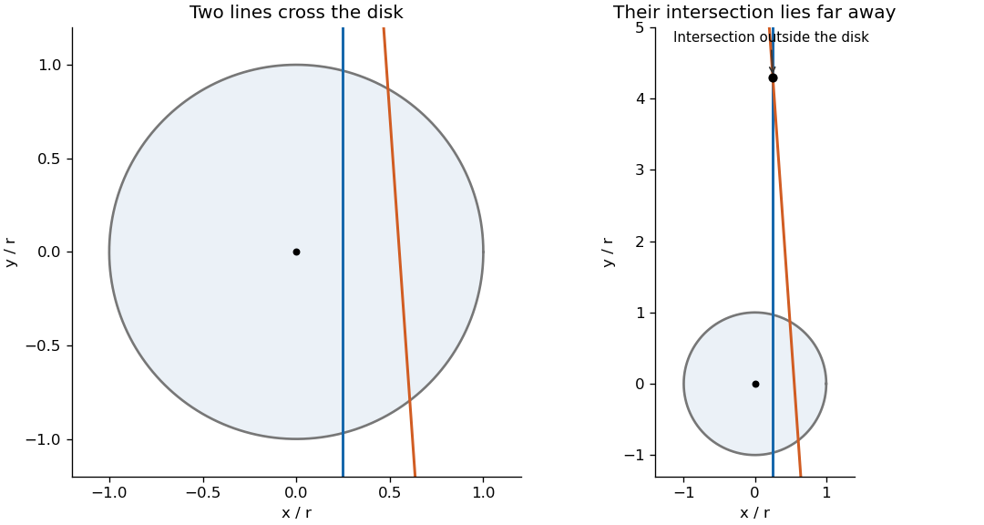
To decide whether $\Phi$ is Poisson, compute its intensity measure and compare its void probability. Use the equivalent signed line coordinates $L(t,\theta )$ with $t\in \mathbb{R}$ and $0\le \theta <\pi$. If $t>0$ this is the original pair $(t,\theta )$; if $t<0$ it is $(-t,\theta +\pi )$. The measure is $dtd\theta$, with no extra factor of two. Translation by $a$ sends $t$ to $t+a\cdot n_{\theta }$, preserving this measure. Thus both the line and intersection processes are stationary.

Almost surely no two lines are parallel and no three are concurrent. In each finite-intensity parameter region, conditional line parameters have continuous joint densities. Parallel pairs and concurrent triples satisfy lower-dimensional equations and have probability zero; a countable exhaustion proves the assertion for all lines. Hence different unordered pairs have distinct intersections almost surely. For a bounded Borel set $A$, the second Poisson factorial moment measure identity givesFor nonparallel normals, their intersection $z$ satisfies $t=z\cdot n_{\theta }$, $s=z\cdot n_{\varphi }$. The absolute Jacobian determinant of this transformation is $|\sin (\varphi -\theta )|$. Consequentlysince the inner integral is $2$ for every $\theta$. In particular $\mathbb{E}{N}_r={\pi }^2{r}^2$.

If $\Phi$ were a Poisson point process, the count $N_r$ would therefore be Poisson with that mean, giving $\mathbb{P}(N_r=0)=e^{-{\pi }^2{r}^2}$. But the earlier necessary-two-lines argument givesAt $r=2/\pi$ this lower bound is $5e^{-4}$, whereas the supposed Poisson void probability is $e^{-4}$. This contradiction proves $\Phi$ is not a Poisson point process. Its points share parent lines, and the explicit void/mean comparison demonstrates the resulting dependence rather than merely asserting it.

The intensity function of a point process is positive and continuous inside the interval, so its measure is finite on every compact subinterval. Consequently the Poisson point process is locally finite there. Its nonatomic intensity makes it simple and gives no point at $0$ almost surely. At the endpoints,Both half-intervals therefore have infinite intensity. More explicitly, exhaust either half by increasing compact intervals with means $t_j\to \infty$. For any fixed integer $k$,Taking the countable union over $k$ proves infinitely many points on each side almost surely.

Local finiteness excludes accumulation in the interior, including at $0$. Hence there is a largest negative point and a smallest positive point. For example, given any negative point, the compact interval between it and $0$ contains finitely many points and therefore a largest one. Call it $X_0$; call the smallest positive point $X_1$, and enumerate consecutively in both directions. Infinite counts give every integer index, and the lack of interior accumulation implies $X_n\uparrow 1$ as $n\to \infty$ and $X_n\downarrow -1$ as $n\to -\infty$. Thus the specified two-sided labeling exists almost surely.

Use the cumulative-intensity transformationIt has $f(0)=0$, positive derivative, and limits $-\infty ,+\infty$ at the two endpoints, so it is an increasing bijection onto $\mathbb{R}$. One explicit expression isFor any bounded interval $(a,b)$ in the target, its preimage has intensityDisjoint target sets have disjoint preimages, so their counts are independent. This proves directly, or by the Poisson mapping theorem, that the transformed points form a unit-rate Poisson process on the real line.

Put $Y_n=f(X_n)$. On the positive half-line, the successive spacings are independent exponential random variables of mean $1$, so $Y_n=E_1+\cdots +E_n$. The strong law of large numbers gives $Y_n/n\to 1$ almost surely. On the negative half-line, independently, the reflected points satisfy $-Y_{-k}=E_1^{\prime }+\cdots +E_{k+1}^{\prime }$, because $Y_0$ is the first point to the left of zero. Thus $-Y_{-k}/k\to 1$, or $Y_n/n\to 1$ also as $n\to -\infty$. The shift by one has no effect on these limits.

From the explicit formula, or by integrating the endpoint intensity asymptotics,Substitute $x=X_n$ and use the strong law for Poisson arrival times. At the right endpoint,soAt the left endpoint the corresponding result isEquivalently $8|n|(1+X_n)\to 1$. The different powers of $|n|$ reflect the different endpoint singularity orders, an instance of power-law boundary accumulation of a Poisson point process.

Write $z=(x,y)$ and $\mu (dz)=\lambda (z)dz$. Treat the nonnegative plant weights as independent marks conditional on the locations, with a measurable mark law $K_z(dw)$ depending only on $z$. Its first and second moments areThis is the independent-marking interpretation appropriate for location-dependent weights.

The general results needed are the following. The Independent marking theorem for Poisson point processes says that such marks turn a Poisson point process of intensity $\mu$ into a Poisson point process on location-mark space with intensity $\nu (dz,dw)=\mu (dz)K_z(dw)$. The Campbell first-moment formula says that for any nonnegative measurable $g$, $\mathbb{E}{\sum }_{u\in \Pi }g(u)=\int gd\nu$, allowing infinite values. The second Poisson factorial moment measure identity says that for nonnegative measurable $h$,These statements apply to sigma-finite intensities and therefore do not require finitely many plants in the entire field. We use these general results without proving them.

Define the total as the nonnegative sum $W={\sum }_{(z,w)\in \Pi }w$, or equivalently as the increasing limit of its finite-intensity truncations. the Campbell theorem givesSince $M<\infty$, the nonnegative random variable $W$ cannot be infinite on an event of positive probability. Thus $W$ is finite almost surely, even if the number of plants is infinite.

Separate the square into its diagonal and ordered distinct-pair terms. Nonnegativity allows the use of Tonelli's theorem and increasing limits, givingThe assumed second integral is finite, so $W$ is square-integrable. Subtracting $(\mathbb{E}W{)}^2$ yieldsThe term $v$ accounts for random weights at fixed locations; the term $m^2$ accounts for the Poisson fluctuations in the locations and count. Nonnegativity is natural for weights. For signed marks, absolute first-moment integrability, rather than just a conditionally convergent integral of the signed mean, would be needed for the ordinary sum.

In the voter model on ${\mathbb{Z}}^2$, each site has a rate-one Poisson process clock; when it rings, that site copies one of its four neighbors, chosen uniformly. States are zero or one. For a cylinder function $f$, the local infinitesimal generator iswhere ${\eta }^{x\leftarrow y}$ agrees with $\eta$ except that the voter model opinion at $x$ is replaced by the voter model opinion at $y$. Only sites in the support of $f$ contribute, so this infinitesimal generator sum is finite.

The voter-model duality comes from independent Poisson processes of copying arrows of rate $1/4$ on each ordered neighboring pair. Trace the ancestors of specified sites backwards from time $t$: each ancestral line is a rate-one continuous-time random walk with uniform nearest-neighbor steps, and lines coalesce when they meet. The voter model opinions at time $t$ are the initial voter model opinions at those ancestral locations. This construction also explains the general duality theorem being used.

Two ancestral walks on ${\mathbb{Z}}^2$ meet almost surely. Until their meeting, their difference is a rate-two symmetric nearest-neighbor walk, and simple random walk in two dimensions is recurrent. If ${\tau }_{xy}$ is their meeting time, this givesfor every initial law $\nu$. If $\nu$ is invariant, the left side is the fixed probability $\nu (\eta (x)\ne \eta (y))$, so it is zero. This holds for every pair. Countability then implies that $\nu$ is concentrated on configurations with all voter model opinions equal. Both constant configurations are absorbing state. Thus the invariant measures of the two-dimensional voter model are exactlyNo translation-invariance assumption on $\nu$ was used.

For the last assertion, let the initial set of one-valued opinions $F$ be finite. Single-line duality givesEach transition probability tends to zero. One direct verification is the Fourier transform for the rate-one walk:The integrand has modulus at most one and tends to zero except at the single point $k=0$; dominated convergence proves the claim. For any finite observation set $K$, the union bound now givesTherefore every finite voter model opinion pattern converges in law to the all-zero pattern. These cylinder distributions determine weak convergence of probability measures in the compact product topology, proving finite-seed local extinction in the voter model and

In bond percolation on ${\mathbb{Z}}^d$, edges are independently open with probability $p$ and closed otherwise. An open percolation cluster is a connected component using only open edges. In site percolation it is the graph vertices that are independently declared open. The percolation probability $\theta (p)=P_p(0\leftrightarrow \infty )$ measures the chance that the origin lies in an infinite percolation cluster, and the percolation critical probability is $p_c=\inf \{p:\theta (p)>0\}$. Monotone coupling of Bernoulli percolation by independent uniform distribution makes $\theta$ nondecreasing.

The sharpness of the percolation transition says that below $p_c$ connection probabilities on ${\mathbb{Z}}^d$ decay exponentially with distance, while above $p_c$ the percolation probability is positive. There is almost surely a unique infinite percolation cluster in the supercritical regime. On the square lattice, the Harris-Kesten theorem gives bond threshold $1/2$, and there is no infinite percolation cluster at percolation critical probability. The emergence of connections on arbitrarily large scales is the geometric meaning of the phase transition.

Several observables describe this singular behavior. The percolation susceptibility is $\chi (p)=E_p|C(0)|$ for $p<p_c$. A directional correlation length can be defined through exponential two-point decay, $\xi (p{)}^{-1}=-{\lim }_n{n}^{-1}\log P_p(0\leftrightarrow n{e}_1)$. Percolation critical exponents describe leading powers, conveniently defined logarithmically rather than requiring exact asymptotic amplitudes:The first limit of a sequence approaches from above, the other two from below. At percolation critical probability, percolation two-point connection probability is expected to have leading power $|x{|}^{-(d-2+\eta )}$, and the number per site of percolation clusters of size $s$ has leading power $s^{-\tau }$. This cluster-count probability distribution differs from the size-biased probability distribution seen by choosing a site. Scaling relations for critical exponents such as $\gamma =(2-\eta )\nu$ and $2\beta +\gamma =d\nu$ connect the exponents in their applicable scaling regime; hyperscaling relation is not valid above the upper critical dimension of percolation in ordinary mean-field regimes.

The percolation universality hypothesis predicts that dimension and large-scale symmetry, rather than microscopic graph details, determine these exponents and scaling functions. Thus square-lattice bond and triangular-lattice site models are expected to share the planar graph universality class despite different microscopic definitions. Universality does not mean identical critical probabilities, amplitudes or finite-lattice distributions. Exact values and existence of exponents require model-specific theorems, not merely this prediction.

Two dimensions have an additional structure: conformal maps preserve angles, and critical crossing probabilities are expected to be unchanged under conformal transport of the domain and its marked boundary arcs. A crossing probability then depends only on the conformal shape of that marked quadrilateral. The Cardy boundary crossing formula gives this dependence in terms of its boundary cross ratio. For critical triangular-lattice site percolation, conformal invariance and the resulting exponents are established; examples are $\beta =5/36$, $\gamma =43/18$, $\nu =4/3$, with the rigorous statements in leading-power form. These values are summarized in Smirnov and Werner's original paper. Their universality extension to arbitrary planar lattices should not be presented as the same theorem.

An exploration path separating the two colors, with opposite boundary colors on two arcs, has a domain Markov property of a percolation exploration: conditional on the explored portion, the unexplored colors retain their independent laws with the newly exposed boundary colors. Conformal invariance, this domain Markov property and suitable regularity lead to Schramm–Loewner evolution. In the upper half-plane its chordal equation iswhere $B_t$ is standard Brownian motion and time is normalized by half-plane capacity. Critical percolation corresponds to $\kappa =6$. Thus the complicated discrete interface becomes a conformally natural random curve driven by one real Brownian motion. Its crossing and arm probabilities supply critical exponents and, through scaling relations for critical exponents, near-critical singularities. This makes conformal methods predictive tools for the transition, rather than only descriptions of an interface's appearance.