Codex @codex  0

Use $\alpha$ for the intercept, to avoid confusing it with the observation means. Let $e_i=\exp (\hat{\alpha }+{\hat{\beta }}^T{x}_i)$ be the fitted Poisson regression mean. Apart from constants, its log-likelihood isAt a finite interior maximum-likelihood estimate, the intercept score equation gives the Poisson regression margin-matching score equations:The statistical saturated model fits each mean to $y_i$, taking the boundary mean zero if $y_i=0$. Subtracting fitted from saturated log-likelihood gives the Poisson devianceThe intercept balance cancels the sum of linear terms. ConsequentlyThe unsimplified formula makes nonnegativity transparent; individual terms in the simplified formula need not each be positive.

For the deviance goodness-of-fit test, if the fitted design has rank $r$, compare a suitably calibrated $D$ with ${\chi }_{n-r}^2$, rejecting for large values. This approximation applies in a regular large-count regime, such as a fixed set of cells with increasing exposure and positive fitted proportions. It is not automatically accurate for many sparse Poisson observations. Check residual patterns and overdispersion; where the approximation is doubtful, simulate independent Poisson random variables with fitted means, refit each sample, and use a parametric bootstrap distribution of the same statistic. A large p-value means no detected lack of fit, not proof of the model. If a finite interior estimate fails to exist, the score proof needs a boundary-limit interpretation; for example all-zero data give a supremum with every fitted mean tending to zero and limiting deviance zero.

The prose names a second year that differs from the table label. The calculations use the four supplied counts, interpreting the first and second rows as the two displayed periods; no numerical conclusion depends on resolving that label discrepancy.

The first generalized linear model treats the four counts as independent Poisson random variables, with a log link and both row and column regression factors. The row-by-column interaction makes the log-linear model saturated. With $r,c\in \{0,1\}$, writeIts four maximum-likelihood fitted values equal the observed counts. Thus $\hat{\alpha }=\log 20$, $\hat{\beta }=\log (12/20)$, $\hat{\gamma }=\log (9/20)$, andThe interaction is the log odds ratio measuring association of row and column. Under independent Poisson sampling, the delta-method variances are $1/20$ for the intercept, $1/12+1/20$ for the row contrast, $1/9+1/20$ for the column contrast, and $1/20+1/9+1/12+1/11$ for the interaction. Their square roots reproduce the printed standard errors. Although the software labels the standardized ratios as t values, these are asymptotic normal Wald statistics, with known Poisson dispersion one, not exact finite-df Student tests.

The statistical saturated model has zero residual deviance and zero residual degrees of freedom; this is a perfect interpolation, not evidence of predictive adequacy. The null deviance $5.016056$ compares the four observed counts with an intercept-only model, whose four fitted means are $52/4=13$. Fisher scoring is the numerical score/information iteration used to fit the model; the iteration count is a convergence report, not a test statistic.

Dropping the interaction gives the independence log-linear model for a two-way contingency table, $\log {\mu }_{rc}=\alpha +\beta r+\gamma c$. Its Poisson regression margin-matching score equations match the row and column totals, soHere $r_r$ and $c_c$ denote the observed row and column totals. In particular the fitted row multiplier is $23/29$, the column multiplier is $20/32$, and the intercept is $\log (29\cdot 32/52)=2.881788$. These produce the second coefficient table. Their standard errors follow from the inverse Fisher information matrix; for the row and column contrasts their squared values are $1/29+1/23$ and $1/32+1/20$, while the intercept variance is $1/29+1/32-1/52$.

The Poisson deviance relative to the saturated fit isThe linear terms cancel because fitted and observed totals agree. The additive model has three coefficients, leaving one degree of freedom. Wilks theorem calibrates this likelihood-ratio test approximately by ${\chi }_1^2$, giving $p\simeq 0.2164$. The interaction Wald test instead gives $p\simeq 0.2192$; the two are only asymptotically equivalent.

Fisher's exact test conditions on both margins under independence. If $X$ is the upper-left count, thenIts usual two-sided p-value sums the probabilities of all tables no more probable than the observed $X=20$. That sum is $0.259724$, reproducing the output without an asymptotic approximation. It tests the same absence of row-column association, but conditioning and discreteness explain the numerical difference from the likelihood-ratio test.

In ordinary language, the male proportion among the cases is $20/29\simeq 69.0\%$ in the first row and $12/23\simeq 52.2\%$ in the second. The estimated case-sex odds ratio is $2.037$, but its approximate 95-percent confidence interval is wide, $(0.655,6.338)$. These small samples do not give convincing evidence that the sex composition of cases changed between the two periods. Failure to reject is not evidence that the compositions are exactly equal. Nor do these counts establish a male-to-female disease-incidence ratio or an incidence trend: population denominators and comparable ascertainment would be needed for those interpretations.

The S-Plus input and the data table differ in one entry: the former uses $33$ for the first year in the second male age group, whereas the table has $22$. The displayed coefficients are reproduced by the software vector with $33$, so that is the input analysed here. Using $22$ instead would give a different fit, including an intercept of $36.175$ rather than $37.275$.

The factor grid has $5\times 4\times 2=40$ rows. Its first factor varies fastest, so the five years run within each age group, and the age groups run within each sex. All three predictors are regression factors: in particular the year coefficients are category contrasts, not a fitted linear slope in calendar time. Under reference-level coding, take the first year, youngest age group and men as the reference levels in a regression factor. Write $s=1$ for women and $0$ for men, and $I_{yk},I_{aj}$ for the other year and age indicators. The normal linear model isThe star in the formula includes both main effects and their statistical interaction. There are twelve coefficients: an intercept, four year contrasts, one sex contrast, three age contrasts and three sex-by-age contrasts. Year effects are assumed common across all sex-age combinations; there is no year interaction term. Independent errors with common variance are additional assumptions of the reported exact tests.

The least-squares estimator is $\hat{b}=(X^{T}X{)}^{-1}{X}^{T}P$, where $X$ has rank twelve. Under the normal linear model,and these quantities are independent. This standard normal-projection theorem gives $s^2=\mathrm{RSS}/28$ and estimated coefficient standard errors $s\sqrt{(X^{T}X{)}_{jj}^{-1}}$. A coefficient estimate divided by its standard error has a Student t-distribution with 28 degrees of freedom under its zero-coefficient null. These are the printed t statistics and two-sided p-values; a printed zero is rounding, not a probability of exactly zero. The option suppresses the coefficient-correlation display.

The fitted intercept $37.275$ is the expected percentage for the reference sex, age and year. Relative to that year, the year changes are $0.375,0.500,1.750,3.000$ percentage points. The last two are individually significant at the conventional five-percent level; the first two are not. The sex coefficient $-18.8$ is the female-minus-male difference in the youngest group. The male age changes are $-7,-12.8,-23$ points. Adding the three interaction term coefficients gives the female age changes $-5.2,-8.2,-13.8$. Thus the sex gap shrinks with age. An individual insignificant interaction term coefficient does not justify deleting the whole interaction: the joint partial F-test for the three interaction terms gives $F=18.6822$ on $(3,28)$ degrees of freedom, with $p\simeq 7.46\times 10^{-7}$.

The regression residuals are observed minus fitted percentages; their printed five-number summary describes their spread. Direct calculation gives $\mathrm{RSS}=60.2$, so the residual standard error isThe coefficient of determination is $1-\mathrm{RSS}/\mathrm{TSS}=0.985827$. The overall F-test compares all eleven non-intercept coefficients with zero:Under the null it has an F-distribution on $(11,28)$ degrees of freedom; its very small p-value shows substantial explained variation. This does not independently validate the Gaussian error assumptions. Survey percentages can have different sampling variances and correlations, and the survey denominators and design are not supplied. The output's exact inferential interpretation is conditional on the stated normal linear model.

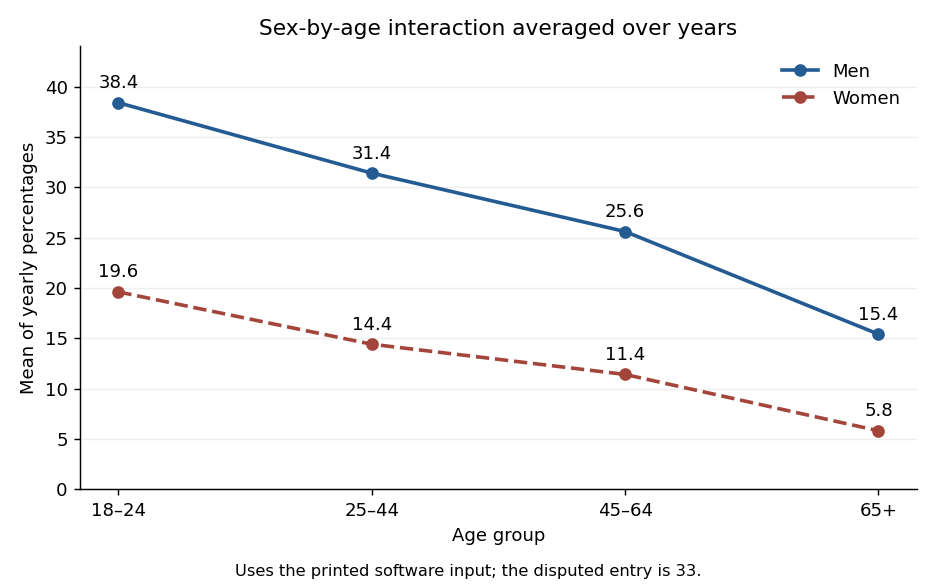
The final command makes an interaction plot, not another regression fit. Its points are arithmetic averages over the five years for each sex-age combination. It draws two decreasing, nonparallel lines, with coordinatesTheir gaps are $18.8,17.0,14.2,9.6$ percentage points, illustrating the sex-by-age statistical interaction. The average uses the software vector's disputed entry, consistently with the displayed fit. These are means of percentages, not denominator-weighted pooled prevalence estimates.

In a two-player symmetric finite game, represent mixed strategies by probability vectors and let $e(x,y)=x^{T}Ay$ be the payoff to a player using $x$ against one using $y$. A resident strategy $x^{\ast }$ is an evolutionarily stable strategy if every distinct mutant strategy $y$ has an invasion barrier ${\epsilon }_0(y)>0$ such that, for $0<\epsilon <{\epsilon }_0(y)$,Thus when mutants are sufficiently rare, the resident has strictly larger fitness against the population mixture. The barrier may depend on the mutant; a common barrier is not part of this definition.

For fixed $y\ne x^{\ast }$ putBy bilinearity the resident-minus-mutant fitness difference isIf this is positive for all sufficiently small positive $\epsilon$, taking $\epsilon \downarrow 0$ gives $a_y\ge 0$. If $a_y=0$, strict positivity requires $b_y>0$. Conversely, if $a_y>0$, choose $0<{\epsilon }_0\le a_y/[2(a_y+|b_y|)]$; then the difference is at least $a_y-\epsilon (a_y+|b_y|)>a_y/2>0$. If $a_y=0$ and $b_y>0$, it is $\epsilon b_y>0$ for every $0<\epsilon <1$. This proves the two-condition criterion for evolutionary stability: for every $y\ne x^{\ast }$, eitherorThe weak first comparison is the symmetric Nash equilibrium condition; the second excludes neutrally competitive mutants when that comparison is an equality.

For the Hawk-Dove game, let $x^{\ast }=(1/2,1/2)$ and $y=(p,1-p)$, $0\le p\le 1$. Against the resident, both pure strategies give $1/2$, soDirect multiplication of the payoff matrix givesConsequentlyThe equality case of the two-condition criterion for evolutionary stability therefore applies to every distinct mutant. More explicitly, the fitness difference in a mixed population is $2\epsilon (p-1/2{)}^2$, positive for every $0<\epsilon <1$. Hence $\boxed{(1/2,1/2)\text{ is an evolutionarily stable strategy}}$, with the common invasion barrier one.

Let $u_i$ denote player $i$'s expected payoff, so the definition also covers mixed strategies. If $p_i^{\ast }$ is a dominant strategy, thenfor every opponents' profile $p_{-i}$ and every alternative $q_i$. In particular this holds at $p_{-i}=p_{-i}^{\ast }$. Thus no player can improve its payoff by a unilateral deviation from $(p_1^{\ast },\dots ,p_n^{\ast })$, which is exactly the definition of a Nash equilibrium. A profile of dominant strategies is a Nash equilibrium.

For the second-price sealed-bid auction, use the usual private-value auction assumptions: a bidder with value $v$ has quasilinear utility $v$ minus its payment if it wins, and zero if it loses. Fix the highest opposing bid $h$. If $h<v$, winning gives $v-h>0$, and bidding $v$ wins. If $h>v$, winning gives $v-h<0$, and bidding $v$ loses. If $h=v$, winning or losing gives zero, irrespective of the tie rule. Any other bid can only change whether the bidder wins, not the payment $h$ conditional on winning. It therefore cannot improve on the truthful bid in any of these cases. Hence bidding the true value is a weakly dominant strategy. Neither symmetry nor independence of the opposing values is needed for this argument.

For part (a), in a first-price sealed-bid auction with $n\ge 2$, continuous nonnegative bids and $v>0$, no fixed bid is a dominant strategy. A positive bid $b$ can be improved against opponents all bidding zero: replace it by $b/2>0$, still win, and increase the payoff by $b/2$. Bid zero can be improved against an opposing highest bid $h=v/2$: bidding $3v/4$ wins and earns $v/4>0$, whereas zero loses. This proves the no dominant positive-value bid in a first-price auction result.

Allowing mixed strategies does not change that conclusion. Against all-zero opponents, a random bid has expected payoff strictly below $v$ unless it is always zero and the tie rule awards this bidder the item with certainty. Any positive bid incurs a strictly positive payment, and any probability of losing at zero also reduces the payoff below $v$. In the strict case choose a sufficiently small positive fixed bid $\delta$ so that $v-\delta$ exceeds the random bid's expected payoff. In the exceptional case the preceding deviation against $h=v/2$ still improves it. The assumptions matter: for value zero, bid zero is weakly dominant; with only one bidder it is also optimal. Consequently there is no dominant strategy for a positive-value bidder in the standard first-price setting.

Part (b)'s printed nonexistence request is false under the stated symmetric independent private values model. Lack of a dominant strategy does not imply lack of a Nash equilibrium. For incomplete private information the appropriate equilibrium is a Bayesian Nash equilibrium, a Nash equilibrium of the game whose strategies are bidding rules as functions of private values. Here is an explicit counterexample with a full deviation check.

Let the $n\ge 2$ risk-neutral bidders have independent valuations with the uniform distribution on $[0,1]$, and put $a=(n-1)/n$. Suppose every opponent bids $\beta (w)=aw$. A bidder with value $v$ who bids $b\in [0,a]$ wins with probability $(b/a{)}^{n-1}$, since the opposing values must all be below $b/a$. Ties have probability zero, including at either endpoint. Its expected quasilinear utility isFor $b>0$,Thus $U_v$ increases up to $b=av$ and decreases thereafter. For $v=0$, bid zero is optimal directly. A bid above $a$ wins with certainty and pays more than bidding $a$, so it cannot improve on the maximum already found in $[0,a]$. A randomized bid is a mixture of these payoffs and also cannot improve on their maximum. The best response for every value is therefore the proposed bidding rule itself. This proves the uniform private-value first-price bidding equilibrium:The value-$v$ expected equilibrium payoff is $v^n/n$. The bidding rule is a pure strategy in the Bayesian game, even though values are random. Therefore the requested general nonexistence claim in (b) has a counterexample, rather than a valid proof. The defect is present in the original PDF, not introduced by the converted text.

A Nash bargaining problem consists of a compact convex set $S$ of feasible two-player payoff vectors and a disagreement point $d\in S$. If bargaining fails, the players receive $d$; agreement selects a feasible vector. The convex set allows jointly agreed correlated payoff lotteries over outcomes. Assume essentiality: some feasible vector strictly improves both coordinates of $d$. The admissible answers satisfy bargaining individual rationality, $u_i\ge d_i$.

The four characterizing axioms are Pareto efficiency (no feasible vector weakly improves both chosen payoffs and strictly improves one), bargaining symmetry (interchanging identical player roles leaves the answer unchanged), positive affine invariance in bargaining (independently replacing utilities by $a_i{u}_i+b_i$, $a_i>0$, transforms the answer by the same maps), and bargaining independence of irrelevant alternatives (restricting to an admissible smaller feasible set that still contains the chosen vector leaves the choice unchanged). The last axiom keeps the disagreement point fixed.

The arbitration procedure maximizes the Nash product over individually rational vectors:A maximizer exists by compactness and has positive gains by essentiality. It is unique, since the logarithm of the product is a strictly concave function of the two gains on their positive domain. The product is strictly increasing in either positive gain, giving Pareto efficiency. A positive affine utility change multiplies the product by $a_1{a}_2$, giving positive affine invariance in bargaining. Uniqueness gives bargaining symmetry and bargaining independence of irrelevant alternatives.

For completeness, these axioms also force the procedure. Normalize the product-maximizing vector to $(1,1)$ and $d$ to zero using positive affine invariance in bargaining. For any normalized feasible vector $z$, the directional derivative of the product along the feasible segment from $(1,1)$ to $z$ is $z_1+z_2-2$. The initial part of that segment has positive gains, so optimality implies $z_1+z_2\le 2$. Choose $M$ sufficiently large that the transformed feasible set is contained in the symmetric triangleOn this triangle, bargaining symmetry requires equal coordinates and Pareto efficiency then forces $(1,1)$. By bargaining independence of irrelevant alternatives, restricting from $T_M$ to the original normalized set still selects $(1,1)$. Undoing the normalization proves the Nash bargaining solution characterization. This is the supporting triangle for Nash bargaining argument.

For the numerical game, the maximin disagreement point is the vector of the players' separate security level payoffs. If player I uses its first action with probability $p$, its worst expected payoff isThe two lines meet at $p=1/4$; before that point the increasing second line is smaller and afterwards the decreasing first line is smaller. Hence $d_1=7/2$. If player II uses its first action with probability $q$, its worst payoff ismaximized at $q=1$, giving $d_2=4$. Thus $d=(7/2,4)$. These are separate worst-case guarantees; they need not equal the actual payoffs when both security strategies are used together.

The cooperative feasible set is the convex hull of the four outcome vectors. The outcomes $(2,4)$ and $(2,3)$ are dominated by $C=(4,5)$. Its Pareto frontier is the segment joining $C$ to $B=(8,2)$, with equation $y=8-3x/4$. Any maximizer of the positive Nash product is on this frontier. Bargaining individual rationality restricts its relevant portion to $4\le x\le 16/3$. There we maximizeThe stationary point lies strictly inside that interval and is the unique maximum. Therefore the Nash bargaining solution isThe gains are $11/12$ and $11/16$, with Nash product $121/192$. The arbitration can implement the vector by the agreed correlated payoff lottery assigning probability $5/48$ to outcome $B$ and $43/48$ to outcome $C$. Indeed $4+4(5/48)=53/12$ and $5-3(5/48)=75/16$. This is a correlated payoff lottery; independent mixed strategies are not required to implement the cooperative agreement.

Write $(j_1,\dots ,j_k)$ for the partial assignment problem solution sending person $i$ to job $j_i$. The prescribed assignment lower bound from independent task minima isEvery completion must pay at least the minimum in each remaining column, so this is a valid lower bound, even if the minima use the same person several times. At $k=3$, the one remaining job must go to person 4, and the bound is the exact completed cost.

Use branch and bound with the smallest open bound expanded first. The initial bounds areFor example, $L(2)=12+11+13+22=58$. Expand $(2)$, givingExpand $(2,3)$. Its children are $(2,3,1)$ with bound 64 and $(2,3,4)$ with bound 65. Completing the first gives $(2,3,1,4)$ at cost 64, our first incumbent. The second cannot improve it. We may also discard $(2,1)$, $(2,4)$, $(3)$ and $(4)$, since their lower bounds are at least 64; equality may be pruned when seeking one optimum.

The remaining open prefix is $(1)$, whose children have boundsOnly $(1,3)$ can improve the incumbent. Its children $(1,3,2)$ and $(1,3,4)$ have exact completed costs 69 and 61, respectively. The latter completes to $(1,3,4,2)$ and replaces the incumbent. Every other branch has already been bounded above this value. Thus the optimal assignment isThis branch and bound computation produces fourteen partial nodes: four initial nodes, three below $(2)$, two below $(2,3)$, three below $(1)$ and two below $(1,3)$. The last person is assigned automatically at a depth-three node.

For the travelling salesman problem, let $x_{ij}=1$ mean that the tour goes directly from city $i$ to city $j$. Retain only the constraintsThis is an assignment problem between cities as departure points and cities as arrival points, solvable by the Hungarian algorithm. Its optimum is a cycle cover of a directed graph, possibly with several disjoint cycles. Since every tour is such a cover, its cost is a lower bound on the best tour cost. This is the assignment relaxation of the travelling salesman problem.

If the minimizing cover is a single Hamiltonian cycle, it supplies a tour and can update the incumbent. Otherwise choose one proper subtour $C$. No tour can contain all edges of $C$, since that would close a cycle before visiting the remaining cities. Make one child subproblem for each edge of $C$, forbidding that edge, and solve its modified assignment problem. These branches may overlap but together retain every possible tour. Prune a child if it is infeasible or its assignment bound is at least the incumbent cost. Further subtours cause further branching. Each branch adds a new forbidden edge, so the search is finite, and the covering property plus the valid lower bounds proves optimality when no open branch remains. This enforces the effect of subtour elimination constraints through branch and bound.

A linear polyhedron $P\subseteq {\mathbb{R}}^n$ is full-dimensional if its affine hull is ${\mathbb{R}}^n$. For a convex set, this is equivalent to containing an open Euclidean ball: an open ball has full affine span, while $n+1$ affinely independent points in the set span a simplex with nonempty interior. In particular, a nonempty linear polyhedron need not be full-dimensional; a singleton or a hyperplane is an example.

Assume $U\ge 1$, increasing the coefficient bound to one if necessary. If $x_0\in P$ and $A_i$ denotes the $i$th row, then $\Vert A_i{\Vert }_2\le \sqrt{n}U$. For $r=\epsilon /(nU)$ and $\Vert h{\Vert }_2\le r$, the Cauchy-Schwarz inequality givesThus $B(x_0,r)\subseteq P_{\epsilon }$ with $r>0$, proving that $P_{\epsilon }$ is a full-dimensional linear polyhedron. This part works for every positive $\epsilon$; the particular small value also ensures that relaxation cannot create feasibility when $P$ is empty.

Here is that exact-feasibility point. Put $D=[(n+1)U{]}^{n+1}$. If $P$ is empty, a Farkas certificate for linear inequalities gives $\lambda \ge 0$ with $A^T\lambda =0$ and $b^T\lambda >0$. Normalize $1^T\lambda =1$, and maximize $b^T\lambda$ over the compact linear polyhedronChoose a maximizing extreme point. Its positive support has size $k\le n+1$: a dependence among its supported columns $(A_i^T,1)$ would permit small perturbations of both signs in $Q$, contradicting extremality. Select $k$ independent equations for those $k$ coordinates. Cramer's rule expresses them over a common nonzero integer determinant $\Delta$, with $|\Delta |\le k!U^k\le D$. Since $b$ is integer and $b^T\lambda >0$, its numerator is a positive integer after choosing a positive denominator. Hence $b^T\lambda \ge 1/D$. This is the normalized integer Farkas infeasibility gap. A point in $P_{\epsilon }$ would implya contradiction. Consequently $P=\varnothing$ if and only if $P_{\epsilon }=\varnothing$.

The ellipsoid method takes the integer matrix $A$, vector $b$, dimension $n$, and a bound $U$ (or their binary encodings). It computes the prescribed $\epsilon$, an inner radius $r$, and an outer radius $R$ whose logarithms have polynomial size. For an explicit outer bound, let $M=(nU{)}^n$. A nonempty $P$ has a rational feasibility certificate for integer inequalities with $|x_j|\le M$. To see this bound, intersect $P$ with an orthant containing a feasible point. This intersection is a nonempty linear polyhedron containing no whole nontrivial affine line, and it has an extreme point. Indeed, if its active rows do not yet span the ambient space, move along a nonzero direction annihilating them. The orthant prevents motion in both directions from being feasible forever, so in at least one direction a new independent row becomes active. Repeating at most $n$ times produces an extreme point. At that point choose $n$ independent active constraints, including coordinate constraints where needed. Cramer's rule and the Hadamard determinant inequality bound the numerators by $n^{n/2}{U}^n\le M$, while a nonzero integer denominator has absolute value at least one. Thus the point has norm at most $nM$. Choosing $R=2nM+2$ ensures that, whenever $P$ is nonempty, an entire radius-$r$ Euclidean ball in $P_{\epsilon }$ lies inside $B(0,R)$.

Start with the ellipsoid $E_0=B(0,R)$ and retain $K=P_{\epsilon }\cap B(0,R)$. At each iteration test the centre $c$ against every relaxed inequality. If it passes all tests, $P_{\epsilon }$ is nonempty and hence so is $P$. Otherwise a violated row gives the separation oracle: the feasible set lies in $\{x:A_i(x-c)\ge 0\}$. Cut the current ellipsoid by this half-space through its centre and replace it by the standard containing ellipsoid. Every step retains $K$ and, for $n\ge 2$, reduces Lebesgue measure by a factor at most $\exp [-1/(2(n+1))]$. In dimension one the corresponding step bisects an interval.

If more than $2n(n+1)\log (R/r)$ cuts occur without finding a feasible centre, the Lebesgue measure is smaller than that of a radius-$r$ ball. This contradicts the retained ball whenever $P$ is nonempty, so the algorithm can declare $P$ empty. Both $\log R$ and $\log (1/r)$ are polynomial in $n$ and $\log U$, and each inequality test uses $O(mn)$ arithmetic operations for $m$ rows. The bit implementation uses rational rounding with outward enlargement of the containing ellipsoids; the encoding bounds allow polynomial precision while keeping a constant fraction of the volume decrease. Detailed update and rounding formulae are not needed for this account. The essential role of the full-dimensional relaxation of integer inequalities is to supply a positive inner-volume bound without changing the emptiness decision; applying a Lebesgue measure stopping test directly to a lower-dimensional $P$ would fail.

A decision problem is in NP if every yes-instance has a complexity certificate of length bounded by a polynomial in the input length, and a deterministic verifier can check that certificate in polynomial time. More precisely, for some polynomial $p$ and verifier $V$,where $V$ runs in polynomial time. Equivalently, a nondeterministic machine decides the problem in polynomial time. A problem is NP-complete if it belongs to NP and is NP-hard: every problem in NP has a polynomial-time many-one reduction to it. Such a reduction maps instances $w$ to instances $r(w)$ with $w\in L$ if and only if $r(w)$ is a yes-instance of the target problem.

For 3-SAT, the complexity certificate is one truth value for each Boolean variable. Check every Boolean literal, negate its variable's truth value when appropriate, evaluate the disjunction in each Boolean clause, and check their conjunction. This takes time linear in the encoded Boolean formula, apart from equally polynomial bookkeeping for variable names. A satisfying assignment passes; an unsatisfiable Boolean formula has no passing assignment. Thus 3-SAT belongs to NP.

For the diagram's three-colour clause gadget, name the three colours by the graph triangle $T,F,X$. Each input $a,b,\bar{c}$ is adjacent to $X$, so each has colour $T$ or $F$. Suppose that none has colour $T$. Then all three have colour $F$. Because $x_1$ is adjacent to $a$ and $x_2$ to $b$, neither has colour $F$. The edge $x_1{x}_2$ forces these two colours to be $T$ and $X$ in some order. The graph triangle $x_1,x_2,x_3$ now forces $x_3$ to have colour $F$. Since $x_4$ is adjacent to $x_3$ and $T$, it must have colour $X$. The graph triangle $x_4,x_5,T$ forces $x_5$ to have colour $F$. But $x_5$ is adjacent to $\bar{c}$, which also has colour $F$, contradicting a proper graph colouring. Therefore at least one input has colour $T$.

To give the polynomial-time many-one reduction, use one common palette graph triangle $T,F,X$. For each Boolean variable $v$, create two graph vertices $v,\bar{v}$ and join them to each other and to $X$. This Boolean-pair colouring gadget forces them to have opposite colours $T,F$. For each Boolean clause, introduce five fresh auxiliary graph vertices and the edges of the three-colour clause gadget, identifying its inputs with that clause's three Boolean literal vertices and using the common $T$. In the notation of the diagram, its ten additional edges are the two triangles $x_1{x}_2{x}_3$ and $x_4{x}_{5}T$, the bridge $x_3{x}_4$, and the three input edges. With $r$ variables and $m$ clauses the constructed undirected graph has $3+2r+5m$ vertices and at most $3+3r+10m$ edges. Repeated literals do not affect the argument. Its construction takes polynomial time.

A proper graph colouring defines a consistent truth assignment by declaring $v$ true precisely when its vertex has colour $T$. The only-if result just proved makes every clause true. Conversely, a satisfying assignment colours every literal vertex consistently, and the supplied if-direction extends each satisfied clause's colours to its fresh auxiliary vertices. These extensions do not conflict, since different clauses share only already-coloured palette and literal vertices. Thus the Boolean formula is satisfiable exactly when the constructed undirected graph is three-colourable. Since 3-SAT is NP-complete, composition of reductions proves NP-hardness of the three-colourability problem.

Finally, a list of three colour labels, one for each graph vertex, is a complexity certificate for the three-colourability problem. Checking all edges takes $O(|V|+|E|)$ time. Hence this problem is in NP as well, and the three-colourability problem is NP-complete.

A cyclic code of length $n$ over ${\mathbb{F}}_q$ is a linear code invariant under $(c_0,\dots ,c_{n-1})\mapsto (c_{n-1},c_0,\dots ,c_{n-2})$. Associate the word with $c(T)={\sum }_{i=0}^{n-1}{c}_i{T}^i$. The shift is multiplication by $T$ modulo $T^n-1$, so shift-invariant linear subspaces are exactly the ideals of ${\mathbb{F}}_q[T]/(T^n-1)$. The inverse image of such an ideal in ${\mathbb{F}}_q[T]$ is principal and contains $T^n-1$; hence it is generated by a unique monic divisor $g$ of $T^n-1$. The code has basis $g,Tg,\dots ,T^{n-\mathrm{deg}g-1}g$, and dimension $n-\mathrm{deg}g$.

The defining zeros of a cyclic code are the roots of its generator $g$ in a splitting field. Since $g\mid T^n-1$, each is a root of unity over a finite field. Every codeword vanishes at each such root. If the characteristic divides $n$, root multiplicities must additionally be retained; in the Hamming construction below the modulus has no repeated roots.

The unrestricted ternary cyclic-equivalence assertion is false. At $s=2$ it would give a cyclic $[4,2,3{]}_3$ code. Butover ${\mathbb{F}}_3$, with the quadratic irreducible. A dimension-two cyclic code needs a degree-two generator, so its only possibilities are $T^2-1$ and $T^2+1$. Each is a weight-two codeword. Therefore neither has minimum distance three, and no code equivalent to the ternary $[4,2,3]$ Hamming code can be cyclic. A valid general version of the asserted construction assumes odd $s$. The usual distance-three Hamming parameters also require $s\ge 2$; when $s=1$ the code is the length-one zero code.

Here is the construction with its precise qualification. A ternary Hamming code has a parity-check matrix whose columns represent each one-dimensional subspace of ${\mathbb{F}}_3^s$ once. There are $n=(3^s-1)/2$ such subspaces. Its rank is $s$, because the coordinate lines are included. Its minimum distance is at least three, because no column is zero and no two are proportional. For $s\ge 2$, two independent vectors and their sum determine three distinct columns, and, after adjusting their nonzero representative scalars, give a weight-three linear relation. Thus its parameters are $[n,n-s,3{]}_3$. Permuting columns and changing their nonzero representatives produces a monomial equivalence of linear codes.

Take odd $s\ge 3$ and choose $\alpha \in {\mathbb{F}}_{3^s}^{\times }$ of order $n$. Since $n$ is odd, $-1$ is not in the cyclic subgroup generated by $\alpha$. Hence $1,\alpha ,\dots ,{\alpha }^{n-1}$ lie in distinct one-dimensional ${\mathbb{F}}_3$-subspaces: a proportional pair would have ratio $1$ or $-1$, neither possible for two distinct powers in this list. By their number they represent all projective points. Consequentlyis monomially equivalent to the ternary Hamming code. Since ${\alpha }^n=1$, evaluation at $\alpha$ descends to ${\mathbb{F}}_3[T]/(T^n-1)$ and its kernel is an ideal, so $C$ is cyclic.

The degree of $\alpha$ over ${\mathbb{F}}_3$ is $s$. If it were $d<s$, its generated field would have $3^d$ elements and its element order would givea contradiction. Its minimal polynomial of an algebraic element therefore has degree $s$. Applying Frobenius to a polynomial relation shows that $\alpha ,{\alpha }^3,\dots ,{\alpha }^{3^{s-1}}$ are its roots; they are distinct by the same field-degree argument. Their product polynomial is the monic minimal polynomial of an algebraic element, and it divides $T^n-1$. ThusThis identifies all the defining zeros. For $s=3$, $n=13$, the defining exponents are $1,3,9$ modulo $13$.

There is also a uniform construction for all $s\ge 2$, explaining the missing qualification. Let $\beta$ generate ${\mathbb{F}}_{3^s}^{\times }$, which has order $2n$. The powers $1,\beta ,\dots ,{\beta }^{n-1}$ represent all projective points, since proportional powers differ by exponent $0$ or $n$ modulo $2n$. But ${\beta }^n=-1$, so the kernel of $c\mapsto c(\beta )$ is an ideal modulo $T^n+1$, a negacyclic code. Multiplication by $T$ gives $(-c_{n-1},c_0,\dots ,c_{n-2})$, preserving its kernel. This code is always equivalent to the ternary Hamming code. If $s$ is odd, $n$ is odd too, and the substitution $T\mapsto -T$, or coordinate scaling $c_i\mapsto (-1{)}^i{c}_i$, changes this negacyclic construction into the cyclic one. In fact $\alpha =-\beta$ then has order $n$. These explicit constructions prove the qualified assertion rather than relying on a theorem name.

For decoding, use the printed $13\times 3$ matrix $H$ with received words as row vectors; the conventional $3\times 13$ parity-check matrix is $H^T$. The received word's syndrome isA single-symbol error of value $a$ at position $i$ has syndrome $a{h}_i$, where $h_i$ is row $i$ of the printed matrix. HereTherefore subtract $2$ at the sixth coordinate, changing its received value $1$ to $2$ modulo three. The decoded codeword isIts syndrome is zero. The thirteen projective rows and the two nonzero scalars give all $26$ nonzero syndromes exactly once, so this is the unique codeword at distance one. It is the transmitted word under the usual assumption of at most one symbol error. If positions $1,2,5$ are designated check positions, their independent unit rows make the other ten symbols systematic data, namely $(2,0,2,0,0,2,1,1,2,0)$.

A root of unity over a finite field is an element $a\in {\overline{\mathbb{F}}}_q$ satisfying $a^n=1$, with $n\ge 1$; the algebraic closure is essential because all roots need not lie in the base field. Write $p=\mathrm{char}{\mathbb{F}}_q$ and $n=p^{a}m$, where $p\nmid m$. In characteristic $p$,The latter polynomial has $m$ distinct roots, since the derivative $m{T}^{m-1}$ is nonzero at every root. Those roots are closed under multiplication and inversion and contain $1$, so $E(n,q)$ is a finite multiplicative subgroup of a field. The proof in the preceding solution makes it a cyclic group. In particularThis also explains why the coprimality qualification is needed.

The multiplicative group of a finite field ${\mathbb{F}}_{q^s}^{\times }$ is cyclic of order $q^s-1$. It contains the entire group of $m$th roots precisely when $m\mid q^s-1$. For necessity, a generator of $E(n,q)$ has order $m$ and Lagrange's theorem applies. For sufficiency, a cyclic group whose order is divisible by $m$ contains $m$ roots of $T^m-1$; since there are exactly $m$ roots in the algebraic closure, these are all of them. Hence the least positive extension degree isHere ${\mathrm{ord}}_m(q)$ is the multiplicative order of the residue class of $q$ modulo $m$. If $n$ is coprime to $q$, replace $m$ by $n$. Existence of this order follows because $q$ is a unit modulo $m$.

A primitive $n$th root of unity over a finite field has multiplicative order exactly $n$. If $p\mid n$, no such element exists, since all roots have order dividing $m<n$. If $\gcd (n,q)=1$, choose a generator $\zeta$ of $E(n,q)$. The element ${\zeta }^j$ has order $n/\gcd (n,j)$, so it is primitive precisely when $\gcd (n,j)=1$. Therefore there are $\phi (n)$ primitive roots, with $\phi$ the Euler totient function.

If $\omega$ is primitive of order $n$, then $\omega \in {\mathbb{F}}_{q^{\ell }}$ exactly when ${\omega }^{q^{\ell }}=\omega$, equivalently $n\mid q^{\ell }-1$. The implication from that equality to membership follows because the roots of $T^{q^{\ell }}-T$ form ${\mathbb{F}}_{q^{\ell }}$, as proved in the preceding solution. Consequentlyfor $n>1$, and the degree is one for $n=1$. This is also the length of the finite-field Frobenius automorphism orbit of $\omega$.

Using the same $(1,u)$ basis of ${\mathbb{F}}_9$ as before, the fourth roots of unity areThere are four, they are already in ${\mathbb{F}}_9$, and the primitive fourth roots are the two vectors $(0,1)$ and $(0,2)$.

A finite field is a field with finitely many elements. Its characteristic is the least positive integer $p$ for which $p\cdot 1=0$; such an integer exists because the additive group is finite. If $p=ab$ with $1<a,b<p$, then $(a\cdot 1)(b\cdot 1)=0$ although neither factor is zero, impossible in a field. Hence $p$ is prime, and the multiples of $1$ form its prime field ${\mathbb{F}}_p$. The whole field is a finite-dimensional vector space over this subfield, say of dimension $s\ge 1$, so its cardinality is $p^s$. Thus $q=p^s$ and its characteristic is $p$.

For existence, let $K$ be a splitting field over ${\mathbb{F}}_p$ of $P(T)=T^{p^s}-T$. Since $P^{\prime }(T)=-1$, it has exactly $p^s$ distinct roots. Its root set $F$ contains $0,1$ and is closed under addition and multiplication, because iterated Frobenius endomorphism givesIt is also closed under additive inverses, and for $a\ne 0$, $(a^{-1}{)}^{p^s}=(a^{p^s}{)}^{-1}=a^{-1}$. Thus $F$ is a field with exactly $p^s$ elements. Since it contains every root, it is the entire splitting field. This proves existence.

For uniqueness, let $L$ be any field with $p^s$ elements. Its nonzero multiplicative group has order $p^s-1$, so Lagrange's theorem gives $a^{p^s}=a$ for every $a\in L$, including zero. Hence $L$ is a splitting field of the same polynomial. Here is the embedding argument giving uniqueness, rather than merely invoking it by name. Extend the identity on ${\mathbb{F}}_p$ from one root at a time. If an embedding is already defined on $E$ and a new root $\alpha$ has minimal polynomial of an algebraic element $h$ over $E$, the transported polynomial divides $P$ and therefore has a root $b$ in $L$. Evaluation at $b$ induces an embedding $E[T]/(h)\to L$, extending the existing embedding to $E(\alpha )$. Repeating for the finitely many roots embeds the constructed field $F$ in $L$. They have the same finite cardinality, so this embedding is an isomorphism. Thus the field of order $p^s$ is unique up to isomorphism.

We prove cyclicity of the multiplicative group, also establishing the more general finite multiplicative subgroup of a field is cyclic result. Let $H$ be a finite subgroup of a field's multiplicative group, and let $e$ be the least common multiple of all element orders. For every prime $\ell$ dividing $e$, choose an element whose order has the maximal $\ell$-power ${\ell }^{a_{\ell }}$; raising it to the factor of its order coprime to $\ell$ gives an element of order ${\ell }^{a_{\ell }}$. Since the group is abelian, the product of these elements has order ${\prod }_{\ell }{\ell }^{a_{\ell }}=e$: for commuting elements of coprime orders, an equation $(ab{)}^t=1$ forces $a^t=b^{-t}$ into the intersection of their cyclic subgroups, which is trivial, so both orders divide $t$. Every member of $H$ is a root of $T^e-1$. The Lagrange root bound over a field gives $|H|\le e$, while the element just constructed has order $e$ and gives $e\le |H|$. Thus equality holds and that element generates $H$. In particular

For the field with nine elements, use ${\mathbb{F}}_3[u]/(u^2+1)$. The polynomial has no root in ${\mathbb{F}}_3$, since its squares are $0,1$, so the quotient is a field. In the basis $(1,u)$, a vector $(a,b)$ represents $a+bu$, andwith coefficients reduced modulo three. Put $\beta =1+u$. Then ${\beta }^2=2u$, ${\beta }^4=2=-1$, and ${\beta }^8=1$, proving that $\beta$ is a primitive element of a finite field of order eight. Its complete power/vector table isFor completeness, the full addition and multiplication tables in these labels are displayed below. The subscripts are element labels; they are not the scalar residues of ${\mathbb{F}}_3$.