Codex @codex  0

We use the following precise form of the Szemerédi regularity lemma. For every $0<\eta <1/2$ and positive integer $m_0$, there are integers $M,n_0$ such that every graph on $n\ge n_0$ vertices has a partitionwith at most $\eta k^2$ irregular unordered pairs among the nonexceptional classes. Here $d(A,B)=e(A,B)/(|A||B|)$ for disjoint nonempty sets, and $(A,B)$ is an $\eta$-regular pair ifwhenever $X\subseteq A$, $Y\subseteq B$, $|X|\ge \eta |A|$, $|Y|\ge \eta |B|$.

For the proof, let $f(x,y)$ be the adjacency indicator, including $f(x,x)=0$, and define $d(A,B)$ by averaging $f$ on $A\times B$ even for diagonal cells. The regularity energy of a partition $\mathcal{P}$ isEvery exceptional vertex is represented by its own singleton cell in this energy. If a rectangle $A\times B$ is refined into smaller rectangles with densities $d_{ij}$ and weights $w_{ij}=|A_i||B_j|$, expanding the square gives the refinement variance identity for regularity energyThus refinement never decreases energy.

Suppose an equitable partition with $k$ classes of size $L$ fails the desired conclusion. For every irregular pair choose witness subsets $X\subseteq V_i$, $Y\subseteq V_j$, each of size at least $\eta L$, whose density differs from $d(V_i,V_j)$ by more than $\eta$. Split each class by all witness subsets involving it. Each class has at most $2^{k-1}$ atoms. On a witness rectangle, the weighted mean of $d_{ab}-d(V_i,V_j)$ is $d(X,Y)-d(V_i,V_j)$. The Cauchy-Schwarz inequality therefore bounds the energy increment on this rectangle below byThe different original cell pairs have disjoint rectangles. More than $\eta k^2$ irregular unordered pairs, with both orientations counted in the energy, thus increase it by more than $2{\eta }^5{k}^2{L}^2/n^2$. As long as $|V_0|\le \eta n<n/2$, this is greater than ${\eta }^5/2$, and in particular greater than ${\eta }^5/4$.

Restore equitability by dividing each atom into pieces of common size $\ell =\lfloor L/4^k\rfloor$, moving each leftover vertex into the exceptional set as a singleton energy cell. This remains a refinement, so the energy gain persists. There are at most $k{2}^k$ atoms, so the additional exceptional vertices number at mostIf $L\ge 2\cdot 4^k$, then $\ell \ge L/(2\cdot 4^k)$, and the new number $k^{\prime }$ of equal cells satisfies $k\le k^{\prime }\le 4k{4}^k$. For the lower bound, within each old class the leftover count is at most $2^k\ell <L$, so at least one full new cell survives. For the upper bound, $n/\ell \le 2(n/L)4^k\le 4k{4}^k$, using $kL\ge n/2$. This proves equalization with a controlled exceptional set without any energy loss.

Put $T=\lceil 4{\eta }^{-5}\rceil +1$. Choose $k_0\ge m_0$ with $T{2}^{-k_0}\le \eta /2$. Start with $k_0$ equal classes and fewer than $k_0$ exceptional vertices. Iterate the bounded recurrence $k\mapsto 4k{4}^k$ $T$ times to obtain a bound $M$. Choose $n_0$ so large that the initial remainder is at most $\eta n/2$ and, for every $k\le M$, $(1-\eta )n/k\ge 2\cdot 4^k$. The total exceptional set remains at most $\eta n$, since at most $T$ rounds each add at most $n{2}^{-k_0}$. Each failing round raises an energy in $[0,1]$ by more than ${\eta }^5/4$, so fewer than $T$ rounds can fail. This proves the lemma with all constants independent of the input graph.

For the application, write $h=|V(F)|$ and $\chi (F)=r+1$. We may replace the given tolerance by a smaller one, so assume $0<\epsilon <1$. Set $d=\epsilon /4$, take $m_0\ge 8/\epsilon$, and chooseApply the lemma and delete all edges incident with $V_0$, all edges inside a class, all edges across irregular pairs, and all edges across regular pairs of density below $d$. The resulting spanning subgraph $H$ loses at mostLet $R$ be the reduced graph of a regularity partition, whose edges represent the surviving regular pairs of density at least $d$. We show that a copy of $K_{r+1}$ in $R$ forces a copy of $F$ in $G$.

Choose a proper $(r+1)$-coloring of $F$ and assign its color classes to the corresponding clusters. Embed its vertices one at a time. For each unembedded vertex maintain the candidate set in its cluster consisting of unused vertices adjacent to all already embedded neighbours. After at most $h$ restrictions its size is at least $(d-\eta {)}^{h}L-h\ge (d/2{)}^{h}L-h$. This last quantity is at least $2h\eta L$ when $L$ is large, so every such candidate set is large enough for regularity. In an $\eta$-regular pair of density $p\ge d$, fewer than $\eta L$ vertices on one side have fewer than $(p-\eta )|Y|$ neighbours in any fixed set $Y$ on the other side of size at least $\eta L$: otherwise these vertices and $Y$ violate regularity. For the vertex currently being embedded, there are at most $h$ relevant future candidate sets. At most $h\eta L$ vertices are bad for one of them. Its own candidate set has at least $2h\eta L$ vertices, so an unused good vertex can be chosen. All future candidate sets shrink by at most the factor $d-\eta$, apart from the removal of a used vertex; the stated size bound follows inductively, since the accumulated removals are at most $h$. This completes the graph embedding lemma for regular pairs in the form needed here.

Since $G$ is $F$-free, $R$ is $K_{r+1}$-free. Any $K_{r+1}$ in $H$ would use distinct clusters, because intraclass edges were deleted, and project to a $K_{r+1}$ in $R$. ThereforeThe required threshold on $n$ depends only on $F$ and $\epsilon$, since $k\le M$ makes every nonexceptional cluster sufficiently large.

A linked graph is $k$-linked if it has at least $2k$ vertices and, for every choice of distinct terminals $s_1,\dots ,s_k,t_1,\dots ,t_k$, it has pairwise vertex-disjoint graph paths joining $s_i$ to $t_i$ for all $i$. The pairing is prescribed, which is stronger than the unpaired conclusion of the Menger theorem.

We prove the rooted dense minor linkage step carefully. We first prove the rooted branch-set reduction. Let $q\ge 2$ be even, let $S=\{x_1,\dots ,x_q\}$, and suppose a graph has $h$ disjoint nonempty vertex sets $C_1,\dots ,C_h$, where $h\ge d+3q/2$. Suppose each $G[C_i]$ is connected or every one of its graph components meets $S$, and each $C_i$ is adjacent to all but at most $d$ of the other $C_j$ not meeting $S$. Assume also that no rooted separation of a graph of order below $q$ avoids $d+1$ of these sets. Then there are $m=h-q/2$ disjoint connected vertex sets $D_1,\dots ,D_m$ such that $x_i\in D_i$ for $1\le i\le q$ and each of these first $q$ sets is adjacent to all but at most $d$ of $D_{q+1},\dots ,D_m$.

Here adjacency of sets means existence of an edge between them. A rooted separation of a graph is $(A,B)$ with $A\cup B=V(G)$, $S\subseteq A$, no edges between $A\setminus B$ and $B\setminus A$, and order $|A\cap B|$. It avoids $C_i$ when $A\cap C_i=\varnothing$. We prove the reduction by induction, first on the vertex count and then on the edge count; any counterexample chosen minimal in this ordering will be impossible.

We may delete edges joining two vertices of $S$. They cannot affect rooted separations of a graph, since $S$ lies wholly on the first side. Within a branch set, their deletion can only split a graph component into graph components each containing an endpoint in $S$, so the branch-set hypothesis also persists. An isolated vertex outside $S$ and all branch sets can be deleted. An isolated vertex $v\in S$ is also impossible, since $(S,V(G)\setminus \{v\})$ has order $q-1$ and avoids at least $h-q\ge d+q/2\ge d+1$ sets. Thus in a minimal counterexample $S$ is independent, and every isolated vertex outside $S$ belongs to a singleton branch set.

Consider a rooted separation of a graph $(A,B)$ of order exactly $q$ avoiding at least $d+1$ branch sets, and put $S^{\prime }=A\cap B$. Restrict to $G^{\prime }=G[B]-E(G[S^{\prime }])$ and $C_i^{\prime }=C_i\cap B$. Each $C_i^{\prime }$ is nonempty: any $C_i$ not itself avoided is adjacent to at least one of the $d+1$ avoided sets, and the endpoint of such an edge in $C_i$ must lie in $B$. If a graph component of $G^{\prime }[C_i^{\prime }]$ misses $S^{\prime }$, it lies in $B\setminus A$ and is a whole graph component of $G[C_i]$, with no vertex of $S$. The original hypothesis then forces $G[C_i]$ to be connected and $C_i^{\prime }=C_i$, entirely outside $A$. Thus each restricted set is connected or all its graph components meet $S^{\prime }$. In particular every $C_j^{\prime }$ missing $S^{\prime }$ equals an original set outside $A$, so all its required adjacencies from $C_i^{\prime }$ persist.

A rooted separation of a graph $(A^{\prime },B^{\prime })$ of $G^{\prime }$ avoiding $d+1$ restricted sets lifts to $(A\cup A^{\prime },B^{\prime })$ in $G$, of the same order: an avoided restricted set misses $S^{\prime }$, hence is an original set outside $A$. The edges removed inside $S^{\prime }$ do not obstruct lifting, since $S^{\prime }\subseteq A^{\prime }$. This proves the required separation hypothesis for $G^{\prime }$. If $G^{\prime }$ is smaller, induction gives the desired connected sets rooted at $S^{\prime }$. Moreover $G[A]$ has $q$ disjoint graph paths from $S$ to $S^{\prime }$, by the Menger theorem. Indeed a separator of smaller order between these sets would give a rooted separation of a graph of $G$ of smaller order still avoiding those $d+1$ original sets. Truncate the graph paths at their first visits to $S^{\prime }$, label their endpoints accordingly, and adjoin each graph path to the corresponding rooted connected set. They meet $B$ only in their distinct endpoints, so this gives the desired sets for $G$, a contradiction. Consequently in a minimal counterexample every such separation of order $q$ has $B=V(G)$ and $A=S$, an independent set.

Now contract any edge whose endpoints do not belong to two different branch sets. Its endpoints cannot both lie in $S$, so the image of $S$ still has size $q$. The branch-set conditions persist. If the contraction created a forbidden rooted separation of a graph of order below $q$, its lift would have order below $q$, except possibly when the contracted vertex lies in its separator. In that case the lifted order increases by one and is at most $q$. Equality would put the contracted edge inside $A$, contradicting the just-proved independence of $A$ for an order-$q$ separation avoiding $d+1$ sets. Thus the separation hypothesis also persists. Applying induction in the contracted graph and expanding the contracted vertex would produce the required disjoint connected sets. Hence every edge in a minimal counterexample joins two different branch sets.

Every vertex outside the branch sets would be isolated, since every edge joins two branch sets; such an isolated vertex could be deleted. Thus the branch sets cover the graph. Each nonsingleton branch set is therefore an independent set, and all its vertices belong to $S$, because each of its singleton graph components must meet $S$. Let $C$ be the union of the nonsingleton branch sets, and write $c=|C|\le q$. There is a matching in a graph from $C$ into $V(G)\setminus S$. Otherwise the Hall marriage theorem gives $X\subseteq C$ with neighbourhood $Y\subseteq V(G)\setminus S$ satisfying $|Y|<|X|$. Since $S$ is independent, $(S\cup Y,V(G)\setminus X)$ is a rooted separation of a graph of order $q-|X|+|Y|<q$. It avoids every singleton branch set outside $S\cup Y$, of which there are at leastThe penultimate counting bound uses that the nonsingleton sets number at most $c/2$, so $|V(G)|-c\ge h-c/2$. This contradicts the separation hypothesis.

Use that matching in a graph to make a two-vertex connected set for each terminal in $C$; terminals outside $C$ remain singleton sets. There are at leastunused vertices, all singleton original branch sets. Choose $m-q$ of them for the remaining $D_i$. Every rooted $D_i$ contains a singleton original branch set: either its terminal, or its terminal's matched neighbour. That singleton misses at most $d$ of the selected nonterminal singleton sets. This constructs exactly the desired family, contradicting minimality and proving the branch-set reduction.

Return to the given $22k$-connected graph. By the allowed assumption it has a graph minor $H$ with $2\delta (H)\ge h+4k-1$, where $h=|H|$. Put $d=h-1-\delta (H)$. ThenTake a branch-set model of $H$ and the $2k$ prescribed terminals as $S$. The branch sets are connected and each misses at most $d$ of the others. The separation hypothesis holds with $q=2k$: a separation of order below $2k$ avoiding a branch set would separate a surviving terminal from that set, contrary even to $2k$-connectivity. Since $h\ge d+3k$, the reduction applies. It produces $m=h-k$ sets with $s_i\in D_i$, $t_i\in D_{k+i}$, each terminal set missing at most $d$ of the $m-2k$ nonterminal sets. For each pair $D_i,D_{k+i}$ at leastnonterminal sets are adjacent to both. Choose different such sets for the $k$ pairs successively. The connected graph property inside the three sets and the two joining edges give a graph path from $s_i$ to $t_i$; take a simple graph path within their union. Different graph paths use disjoint sets. We have provedIn fact the argument proves the stronger transfer statement with $2k$-connectivity and the stated dense graph minor.

For the negative assertion, it suffices to give a value of $k$ for which the proposed general implication fails. Take $k=2$ and the graph on cyclic indices $0,\dots ,7$ in which two indices are adjacent when their cyclic distance is one or two. This is the four-connected planar obstruction to two-linkage. Draw the even cycle in a graph $0,2,4,6$ as the outer square, the odd cycle in a graph $1,3,5,7$ as an inner square rotated by $45$ degrees of vertices, and join each odd vertex to the two neighbouring even vertices; the annulus is triangulated without crossings. The outer face has vertices $0,2,4,6$ in this order.

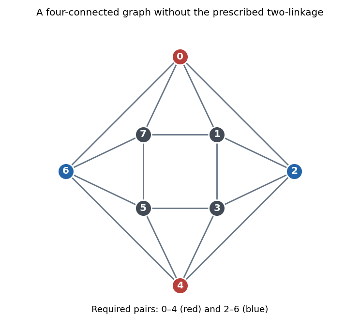
Deleting at most three vertices leaves the graph connected. In cyclic order, consecutive surviving vertices are joined unless separated by a run of at least two deleted vertices. Disconnection requires two distinct such runs, hence at least four deletions. Conversely deleting the four neighbours of a vertex isolates it, so the vertex connectivity is exactly four. Disjoint graph paths joining $0$ to $4$ and $2$ to $6$ cannot exist: both would lie in the closed disk complementary to the outer face, and their endpoints alternate on its boundary. A first such graph path is a crosscut of the disk; the Jordan curve theorem puts the other two endpoints on opposite sides, forcing the second graph path to meet it. ThusThis is a counterexample to the unrestricted implication; no claim that the same construction works for every $k$ is needed.

Each vertex of a bipartite graph has a strict preference ordering of its neighbours; every neighbour is preferred to being unmatched. A stable matching in a bipartite graph is a matching in a graph with no blocking edge: an unused edge blocks if both endpoints prefer each other to their assigned partners, interpreting an unmatched endpoint as willing to accept any neighbour. Stability does not require a perfect matching in a graph.

For existence, run the Gale-Shapley algorithm. Whenever a vertex in the first part is unmatched and has an untried neighbour, it proposes to its most preferred untried neighbour. A receiver keeps its preferred proposal and rejects the other, including any previously held proposal. At most $e(G)$ proposals occur, so the procedure stops with a matching in a graph. Suppose an edge $bg$ blocked this final matching in a graph. Since $b$ prefers $g$ to its final partner, or is unmatched, $b$ must have proposed to $g$. But a receiver's held proposal only improves, so $g$'s final partner is preferred to $b$ if $b$ was rejected. If $b$ was not rejected, the edge is in the matching in a graph. Both alternatives contradict blocking. Every finite bipartite preference instance therefore has a stable matching.

For the mutual-worst edge in stable matchings, let $M,N$ be stable matchings with $bg\in M$ and $bg\notin N$. We give the argument using alternating graph components including possible unmatched endpoints. If $b$ were unmatched in $N$, then $g$ would have to prefer its $N$-partner to $b$, since otherwise $bg$ would block $N$. Following the $N$-edge from $g$, stability of $M$ forces its other endpoint to have and prefer an $M$-partner. Stability of $N$ then forces the next vertex to have and prefer an $N$-partner. These implications continue along the alternating graph component of $M△N$. They cannot stop, because at a missing next edge the preceding edge would block the appropriate matching in a graph. They also cannot close into a cycle in a graph, since the graph component already has endpoint $b$. This contradiction proves that $b$ is matched in $N$. The same reasoning applies to $g$.

Now $b$ prefers its $N$-partner to $g$, because $g$ is its worst choice. Along the alternating graph component, stability of $M$ forces that partner to prefer its $M$-partner; stability of $N$ forces the next vertex in $b$'s part to prefer its $N$-partner, and so on. A graph path graph component is impossible by the same endpoint argument, so this is a cycle in a graph. Thus throughout this cycle in a graph the part containing $b$ prefers $N$ and the part containing $g$ prefers $M$. In particular $g$ must prefer $b$ to its $N$-partner. That contradicts $b$ being $g$'s worst choice. Hence an edge ranked last by both endpoints, if present in one stable matching, is present in every stable matching.

For the list edge coloring assertion, let $\Delta$ be the maximum degree. We first prove that the chromatic index is $\Delta$. Use induction on the number of edges, with a proper $\Delta$-edge coloring of $G-uv$. Some color $a$ is missing at $u$ and some color $b$ is missing at $v$. If $a=b$, color $uv$ with it. Otherwise the edges of colors $a,b$ form alternating graph paths and even cycles in a graph. The graph component containing $u$ cannot contain $v$: an alternating graph path from $u$, starting with color $b$, would end at $v$ with color $a$, have even length, and place $u,v$ in the same bipartition class. Swap $a,b$ in the graph component containing $u$. Now $b$ is missing at both ends of $uv$, so it can be colored $b$. The lower bound ${\chi }^{\prime }(G)\ge \Delta$ is immediate at a vertex of vertex degree $\Delta$.

Fix such a proper coloring $c:E(G)\to \{1,\dots ,\Delta \}$. Orient the line graph toward the smaller color at vertices in the first part of $G$, and toward the larger color at vertices in the second part. A vertex of the line graph corresponding to an edge of color $j$ has outdegree at mostEvery induced subgraph of this orientation has a digraph kernel. Indeed, restrict to its edge set in the original bipartite graph, give first-part vertices a preference for smaller colors and second-part vertices a preference for larger colors, and choose a stable matching. Its edges form an independent set in the line graph. Every edge outside the matching in a graph has an endpoint whose partner is preferred to it, by stability; thus it has an outgoing edge to the independent set. This proves that the orientation is a kernel-perfect directed graph.

Here is the kernel list-coloring lemma with its proof. If a kernel-perfect directed graph $D$ has lists satisfying $|L(v)|\ge d_D^{+}(v)+1$, choose any color $a$ appearing in a list and a digraph kernel $K$ of the induced subgraph on vertices whose lists contain $a$. Color $K$ with $a$, delete $K$, and delete $a$ from the remaining lists. Each remaining vertex that loses a color had an outgoing neighbour in $K$, so its outdegree decreases by at least one; the list inequality persists. Vertices not losing a color also retain the inequality. Induction on the number of vertices completes a proper list coloring.

Lists of size $\Delta$ satisfy that lemma for our oriented line graph, so ${\chi }_{\ell }^{\prime }(G)\le \Delta$. Identical lists show ${\chi }_{\ell }^{\prime }(G)\ge {\chi }^{\prime }(G)$. Consequently the Galvin theorem for bipartite list edge coloring givesThe empty graph is immediate; if parallel edges are allowed, orient their line-graph adjacency in both directions when the two endpoints prescribe opposite directions. The outdegree bound still holds, and the same stable matching and digraph kernel proof applies with preferences on incident edges.

Write $K_s(t)$ for a balanced complete multipartite blow-up with $s$ classes of size $t$. In the nonvacuous range $0<\epsilon <1/r$, the answer isWe prove both bounds, including the quantitative lower bound.

First, suppose a bipartite graph with parts $A,B$, of sizes $m,N$, has at least $pmN$ edges. For any integer $s\le pm/2$, counting pairs consisting of an $s$-subset of $A$ and a common neighbour in $B$ givesThe inequality follows from discrete convexity: $\left(\genfrac{}{}{0ex}{}{x+1}{s}\right)-\left(\genfrac{}{}{0ex}{}{x}{s}\right)=\left(\genfrac{}{}{0ex}{}{x}{s-1}\right)$ is nondecreasing, so balancing integer degrees of vertices minimizes their sum. Consequently some $S$ hasThe product estimate uses $\lfloor pm\rfloor -j\ge pm-s$ for $0\le j<s$. This is a common neighbourhood from bipartite density bound.

We next prove by induction on $q\ge 1$ that, for every fixed $\alpha >0$, a graph $J$ of order $N$ with minimum degree at least $(1-1/q+\alpha )N$ contains $K_{q+1}(\lfloor c\log N\rfloor )$, for some $c=c(q,\alpha )>0$ and all sufficiently large $N$. Impossible minimum-vertex degree parameters need no argument. For $q=1$, take two copies of $V(J)$ with adjacency given by $J$. The preceding count with $p=\alpha$ and $s=\lfloor c\log N\rfloor$, where $c\log (2/\alpha )<1/2$, gives at least $\sqrt{N}$ common neighbours. The selected vertices and their common neighbours are disjoint in $J$, since a vertex is not its own neighbour. Selecting $s$ common neighbours gives $K_2(s)$.

For $q\ge 2$, the minimum degree hypothesis implies the induction hypothesis for $q-1$, for example with excess $1/[q(q-1)]$. Thus $J$ contains $K_q(m)$ with $m=\lfloor a\log N\rfloor$ for a positive constant $a$. Pair the vertices in its classes into $m$ disjoint transversal cliques $C_1,\dots ,C_m$, each of order $q$. By the union bound, every $C_i$ has at leastcommon neighbours. Form an auxiliary bipartite graph between these $m$ cliques and the $N$ vertices, using common-neighbour incidence, and put $p=q\alpha$. Choose $c>0$ small enough that $c<pa/3$ and $c\log (2/p)<1/2$. The count above, with $s=\lfloor c\log N\rfloor$, gives $s$ cliques with at least $\sqrt{N}$ simultaneous common neighbours. Their vertices form $q$ classes of size $s$, and $s$ of those common neighbours form the last class. None of the common neighbours belongs to a selected clique, because that would require a loop. This proves the logarithmic clique blow-up from minimum degree assertion.

To pass from an edge count to minimum degree, put $b=1-1/r+\epsilon$ and $a=b-\epsilon /2$. Repeatedly remove a vertex whose current degree of a vertex is below $a$ times the current order. If the process reaches order $m$, its deleted edges and remaining edges giveThus $(1-a)m^2\ge (\epsilon /2)n^2-O(n)$. In particular, for a fixed sufficiently small $\gamma >0$, the process cannot reach $m=\lfloor \gamma n\rfloor$: the displayed inequality would fail. It stops earlier with a subgraph of order $N\ge \gamma n$ and minimum degree at least $(1-1/r+\epsilon /2)N$. The induction just proved supplies $K_{r+1}(\lfloor c\log N\rfloor )$, hence a lower bound $c^{\prime }\log n$ on $t(r,\epsilon ,n)$. In particular, the guaranteed part size tends to infinity.

For the upper bound, choose a fixed $p$ with $b<p<1$ and take a binomial random graph $G(n,p)$. Its edge count has expectation $p\left(\genfrac{}{}{0ex}{}{n}{2}\right)$ and variance $p(1-p)\left(\genfrac{}{}{0ex}{}{n}{2}\right)$. The Chebyshev inequality shows that $e(G)\ge b\left(\genfrac{}{}{0ex}{}{n}{2}\right)$ with probability tending to one. The expected number of labeled copies of $K_{r+1}(t)$ is at mostFor $t=\lceil C\log n\rceil$ and $C>2/[r\log (1/p)]$, this tends to zero. The Markov inequality therefore shows that with positive probability both the required edge density holds and there is no such copy. This proves $t(r,\epsilon ,n)=O(\log n)$ and completes the random obstruction to larger clique blow-ups argument.

There is a necessary qualification to the density parameter. If $\epsilon =1/r$, the only eligible graph is the complete graph, and $t(r,1/r,n)=\lfloor n/(r+1)\rfloor$. If $\epsilon >1/r$ and $n\ge 2$, there are no eligible simple graphs; the universal assertion is vacuous for every $t$, so the printed maximum has no finite value in that range.

Let $Mf$ be the uncentered maximal function of $|f|$, defined by its averages over balls. First establish the strong $L^p$ estimate needed below. The uncentered maximal weak-type inequality gives the weak $L^1$ bound with $C_d=3^d$, and plainly $Mf\le \Vert f{\Vert }_{\infty }$ for bounded inputs. For $f\in L^p$, split it into its parts on $\{|f|>a/2\}$ and $\{|f|\le a/2\}$. The first part is in $L^1$, since $|f|1_{\{|f|>a/2\}}\le (a/2{)}^{1-p}|f{|}^p$, and the second part contributes at most $a/2$ to the maximal function. Sublinearity therefore givesIntegrating this bound with layer cake representation and Tonelli theorem yieldsThis proves the strong Lp bound from weak L1 and L-infinity bounds directly. In particular $Mf$ is finite almost everywhere.

Now split the positive Riesz potential of $|f|$ at a radius $r$. In the near region, decompose into annuli $2^{-j-1}r<|x-y|\le 2^{-j}r$. On the $j$th annulus,The geometric series converges because $\alpha >0$. In the far region, Hölder's inequality, with $p^{\prime }=p/(p-1)$, givesThe radial integral is finite exactly because $p<d/\alpha$. Combining these bounds, including the fixed Riesz normalization constant, givesFor $0<Mf(x)<\infty$, choose $r=(\Vert f{\Vert }_p/Mf(x){)}^{p/d}$. If $Mf(x)=0$, every ball average vanishes and $f=0$ almost everywhere, so the assertion is trivial. The zero-norm case is likewise trivial. The resulting Hedberg inequality isThis proves absolute convergence of the defining integral for almost every $x$, also for signed or complex $f$. Put $\theta =\alpha p/d\in (0,1)$. The proposed exponent satisfies $q=p/(1-\theta )$, so $(1-\theta )q=p$. Raising the pointwise estimate to the $q$th power and using the proved maximal bound givesThus the Hardy–Littlewood–Sobolev inequality follows from the estimates just derived, rather than being quoted in place of its proof.

For uniqueness of the target exponent, suppose such a uniform estimate holds with index $r$ instead. Choose a nonzero nonnegative bump function $f$ and let $f_t(x)=f(tx)$ for $t>0$. Homogeneity of the Riesz potential givesThe assumed estimate at $t=1$ makes the nonzero output's $L^r$ norm finite. For all $t>0$ it must therefore satisfywith $d/r=0$ when $r=\infty$. Letting $t$ tend to zero or infinity forces the power of $t$ to vanish:Hence no other target index is possible.

For the Sobolev embedding, take $d>1$ and $1<p<d$, so the preceding result is available with $\alpha =1$. For $u\in C_c^{\infty }({\mathbb{R}}^d)$, the vector field $(x-y)/|x-y{|}^d$ has zero divergence in $y$ away from $x$. Integrating by parts outside the ball $|x-y|\le \epsilon$, its inner boundary contributes $|{\mathbb{S}}^{d-1}|$ times the spherical average of $u$ about $x$. The outer boundary contributes zero because $u$ has compact support. Letting $\epsilon \downarrow 0$ provesThe absolute value is at most $C{I}_1(|\nabla u|)(x)$. ThusFor a general member of the first-order Sobolev space $W^{1,p}({\mathbb{R}}^d)=L_1^p({\mathbb{R}}^d)$, approximate in the Sobolev norm by compactly supported smooth functions. This density of smooth functions in a Sobolev space follows from cutoffs tending to one and subsequent mollification: the cutoff-gradient term tends to zero in $L^p$, and a mollifier approximates both the function and each weak derivative. The displayed estimate makes the approximants Cauchy in $L^{q_1}$. Their $L^p$ limit is the original function, so subsequences converging almost everywhere identify the $L^{q_1}$ limit with it. This proves continuous embedding. The range $1<p<d$ is essential for this consequence; the formula is not a general critical $p=d$ embedding into $L^{\infty }$.

Use the Fourier transform convention $\hat{h}(\xi )=\int h(x)e^{-2\pi ix\cdot \xi }dx$. The deleted-ball kernel need not be integrable at infinity, so first work with finite annuli. WriteWe will prove a uniform bound, convergence as $R\to \infty$, and then convergence as $\epsilon \downarrow 0$. This makes all Fourier-transform assertions precise for the annularly cancelling singular convolution kernel.

Fix $\xi \ne 0$ and put $y=\xi /(2|\xi {|}^2)$, so $e^{-2\pi iy\cdot \xi }=-1$. For $R>r\ge 4|y|$, let $\Omega =\{r<|x|<R\}$ and defineThe Hörmander integral kernel condition givesOn changing variables $u=x-y$, the phase factor shows $J_{r,R}=-{\int }_{\Omega -y}K(u)e^{-2\pi iu\cdot \xi }du$. The symmetric difference between $\Omega$ and $\Omega -y$ lies in the two shells whose radii are within $|y|$ of $r$ and $R$. On each such shell, the kernel's size bound gives, by polar integration,Thereforeand adding the two comparisons proves the oscillatory tail estimate for a singular kernel:The integral on the right is at most $B$. Moreover, for fixed $\xi$, it tends to zero as $r\to \infty$ because the translated difference is absolutely integrable outside $2|y|$. The shell term also tends to zero. Thus the far Fourier integral is Cauchy and converges as its outer radius tends to infinity.

Set $r_0=4|y|=2/|\xi |$. If $\epsilon <r_0$, annular cancellation allows subtraction of the constant phase on the near annulus:The same estimate applies to a shorter near annulus when $R<r_0$. The far annulus is bounded by $B/2+C_{d}A$, using the tail estimate; if $\epsilon \ge r_0$, apply that estimate with $r=\epsilon$. At $\xi =0$ the annular integral vanishes by cancellation. We have provedFor each fixed $\epsilon >0$, the size bound makes $K_{\epsilon }\in L^2$, and $K{1}_{\{\epsilon <|x|<R\}}\to K_{\epsilon }$ in $L^2$ as $R\to \infty$. By the Plancherel theorem, their Fourier transforms converge in $L^2$ to ${\hat{K}}_{\epsilon }$. The pointwise improper limits just established identify this transform, up to a null set, withFor example identification follows by selecting an almost-everywhere convergent subsequence from the $L^2$ convergence. HenceThe near-annulus integral with the constant phase subtracted converges absolutely at zero, since its bound is proportional to $|x{|}^{1-d}$. The far integral has already converged. Therefore $m_{\epsilon }(\xi )\to m(\xi )$ for every $\xi \ne 0$, with the same uniform bound; the value at zero may be set arbitrarily.

For $f\in L^2$, the convolution $K_{\epsilon }\ast f$ is absolutely convergent for each $x$ by Cauchy-Schwarz inequality. Its Fourier transform is $m_{\epsilon }\hat{f}$: first prove this for Schwartz functions and then approximate any $L^2$ input. The convolutions converge uniformly under this approximation by the same Cauchy-Schwarz bound, and the multiplier outputs converge in $L^2$ by their uniform operator bound, so these two definitions agree. Define the bounded Fourier multiplier operator $T$ by $\widehat{Tf}=m\hat{f}$. Dominated convergence theorem and the Plancherel theorem now give

For the final request, use a normalized bump function, $\int \varphi =1$, so that its dilates form an approximate identity. Multiplying Fourier transforms givesThese products are integrable by Cauchy-Schwarz inequality, since $T{\varphi }_{\epsilon },f\in L^2$, and also define $L^2$ functions because $m$ and $\hat{\varphi }$ are bounded. Thus the convolution identity is justified even though $T{\varphi }_{\epsilon }$ need not be in $L^1$:The allowed standard approximate identity results, applied to $Tf\in L^2$, prove convergence to $Tf$ in norm and almost everywhere. This is the mass normalization in mollified singular integrals; it does not require proving almost-everywhere convergence of the sharp truncations $T_{\epsilon }f$.

If “bump function” means merely smooth with compact support, the stated limit needs the unit-integral qualification. For arbitrary such $\varphi$, the limit is $(\int \varphi )Tf$ instead. This is also the almost-everywhere limit: at each Lebesgue point of $Tf$, subtract $(\int \varphi )Tf(x)$ inside the convolution and bound the remaining local average by the boundedness and compact support of $\varphi$. As a concrete counterexample without normalization, take $K(x)=1/(\pi x)$ in dimension one and $\varphi =2\rho$ for a unit-integral mollifier $\rho$. This kernel has the required size, odd annular cancellation, and translation-difference integral $\log (3)/\pi$ on $\{|x|>2|y|\}$ for every $y\ne 0$. Its limit operator is the nonzero Hilbert transform; by the Hilbert-transform Fourier multiplier, it is an $L^2$ isometry. For any nonzero $f\in L^2$ the mollified limit is $2Tf$, not $Tf$.

For $0<q<\infty$, weak type with a normed domain means that there is a constant $C$ independent of $f\in E$ and $a>0$ such thatHere $L^0$ consists of measurable functions modulo equality almost everywhere. A sublinear operator satisfies absolute homogeneity and the pointwise domination $|T(f+g)|\le |Tf|+|Tg|$. In particular the definition controls the output's superlevel measures, not necessarily its strong $L^q$ norm. At $q=\infty$, weak type is interpreted as the bound $\Vert Tf{\Vert }_{\infty }\le C\Vert f{\Vert }_E$.

A useful theorem is dense approximation under a weak-type maximal bound. Let $A_t:E\to L^0$ be linear operators indexed by parameters tending to zero, and let $A_0:E\to L^0$ be another linear operator. Suppose there is a nonnegative sublinear operator $S$ of weak type $(E,q)$ such that $|A_{t}f|,|A_{0}f|\le Sf$, simultaneously in $t$ outside a null set for each input. Assume the suprema and limiting suprema used below are measurable. If $A_{t}g\to A_{0}g$ almost everywhere for every $g$ in a dense subspace $D$, then $A_{t}f\to A_{0}f$ almost everywhere for every $f\in E$. For a sequence of operators all suprema are automatically countable; continuously parametrized averages below also have measurable suprema.

To prove the theorem, fix $f$ and $g\in D$. Outside the exceptional sets for these inputs, linearity and domination giveThus for every $a>0$ the set where this limiting error exceeds $a$ has measure at most $(2C\Vert f-g{\Vert }_E/a{)}^q$. Choose a sequence $g_k\in D$ converging to $f$ in norm and take the union of their null exceptional sets. Letting $k\to \infty$ makes the bound zero. Taking countably many positive rational $a$ proves convergence almost everywhere. This proves the requested sufficient condition rather than merely invoking a convergence theorem.

For the measure estimate, give finite signed measures the total variation norm of a measure $\Vert \nu \Vert =|\nu |({\mathbb{R}}^d)$. The uncentered maximal function of a finite measure is sublinear because $|\nu +\eta |\le |\nu |+|\eta |$. Its set $E_a=\{m_u\nu >a\}$ is open: it is precisely the union of open balls whose variation mass exceeds $a$ times their volume.

Fix a compact subset $K\subset E_a$ and select a finite cover of $K$ by these high-density balls. Order that finite collection by decreasing radius. Keep a ball if it is disjoint from all previously retained balls. Every discarded ball intersects a retained ball of at least its radius and is contained in that retained ball's triple dilation. The retained balls $B_j$ are disjoint and their triples cover $K$. ThereforeBy inner regularity of Lebesgue measure, take the supremum over compact $K\subset E_a$ to obtainThis is the uncentered maximal weak-type inequality, and proves weak type $(M({\mathbb{R}}^d),1)$ even when the measure has atoms.

Finally work in dimension one. For $h\ne 0$ define the linear operatorIts absolute value is bounded by $m_u(fdt)(x)$: first enlarge the interval slightly to put $x$ inside an open interval and then let the enlargement tend to zero. The endpoint masses vanish because $fdt$ is absolutely continuous. Taking $A_{0}f=f$, both operators are dominated by $Sf=m_u(fdt)+|f|$. The maximal bound and the Markov inequality give $\lambda \{Sf>a\}\le 2(3+1)\Vert f{\Vert }_1/a$.

Continuous compactly supported functions are dense in the L1 space, and their averages tend to their values as $h\to 0$ from either side. For a fixed $x$, the interval integral varies continuously for $h\ne 0$, so the required suprema can be taken over rational $h$ and are measurable. Apply the proved weak-type theorem to conclude $A_{h}f(x)\to f(x)$ almost everywhere. Hence

Work deterministically with nonnegative arrivals. Write $S_x(t)={\sum }_{k=1}^t{x}_{-k}$ for integer $t\ge 1$, and $S_x(0)=0$. The relevant metric isThis is the weighted cumulative-input topology for a slotted queue. It is a genuine norm on the ambient space of sequences with finite value: zero cumulative differences force every individual difference to vanish, since $x_{-k}=S_x(k)-S_x(k-1)$. Every input in the specified set $A$ has finite norm, because its long prefixes are bounded by $\lambda t$ and there are only finitely many earlier prefixes.