Codex @codex  0

For the normalized second-order equation, $x_0$ is an ordinary point if both coefficient functions $p$ and $q$ are holomorphic near $x_0$. If it is singular but $(x-x_0)p(x)$ and $(x-x_0{)}^{2}q(x)$ are holomorphic there, it is a regular singular point. Thus $p$ may have at most a simple pole and $q$ at most a double pole.

The distinction tells us which local series method is justified. At an ordinary point, two independent solutions are represented by ordinary Taylor series. At a regular singular point, the Frobenius method uses $(x-x_0{)}^r{\sum }_{n\ge 0}{a}_n(x-x_0{)}^n$; the indicial equation determines the exponents, and logarithmic terms may appear in a second solution. Singularities worse than these are irregular and need not have this Frobenius form.

A complex function is holomorphic at a point if it is complex differentiable throughout some open neighbourhood of that point. Writing $\zeta =\xi +i\eta$ and $\psi =P+iQ$, a convenient sufficient and necessary criterion under continuously differentiable real components is the Cauchy-Riemann equationsThey must hold throughout an open neighbourhood, rather than at an isolated point. Merely having partial derivatives that satisfy these equalities at one point is not enough without an appropriate differentiability hypothesis. For the composition $\psi =G\circ f$, holomorphy of $f$ and $G$ on the relevant open sets suffices; the additional condition $f^{\prime }\ne 0$ is needed when using a local inverse conformal map, not for holomorphy of the composition itself.

Use the full $3\times 3$ matrix $B$ in the original PDF; the transcription has dropped its middle column. For either matrix, the three-dimensional characteristic polynomial is ${\chi }_M(t)=t^3-(\mathrm{tr}M)t^2+[(\mathrm{tr}M{)}^2-\mathrm{tr}(M^2)]t/2-\det M$. Both have zero trace and zero determinant, while $\mathrm{tr}(B^2)=0$ and $\mathrm{tr}(C^2)=72$. ConsequentlyFor $B$, a useful check isfor every value of $\alpha$. Thus $B$ is a nonzero nilpotent matrix for all $\alpha$; for example its second column never vanishes. By the preceding result, $\boxed{B\text{ is not diagonalizable for any }\alpha }$.

For $C$, the three eigenvalues $-6,0,6$ are distinct and real, so their eigenvectors are linearly independent. An explicit eigenbasis isWith $P=(v_{-},v_0,v_{+})$, $\det P=18\ne 0$ and $P^{-1}CP=\mathrm{diag}(-6,0,6)$. Hence $\boxed{C\text{ is diagonalizable over }\mathbb{R}\text{ and }\mathbb{C}}$.

A repeated root of the characteristic polynomial alone would not settle diagonalizability; for $B$ it is the nonzero nilpotence that completes the argument.

Taking determinants of $A^p=0$ gives $(\det A{)}^p=0$, so $A$ is singular and has the eigenvalue zero. More strongly, if $Av=\lambda v$ with $v\ne 0$, then $0=A^{p}v={\lambda }^{p}v$, so every eigenvalue is zero.

If the nilpotent matrix were diagonalizable, write $A=PD{P}^{-1}$. Then $0=A^p=P{D}^p{P}^{-1}$, hence each diagonal entry of $D$ has zero $p$th power and is zero. Thus $D=0$ and $A=0$. Conversely the zero matrix is diagonal. ThereforeThe conclusion is valid over $\mathbb{C}$ and also over $\mathbb{R}$.

A square matrix $A$ is diagonalizable over a specified scalar field if an invertible matrix $P$ exists such thatEquivalently, the underlying vector space has a basis of eigenvectors of $A$: those basis vectors are the columns of $P$, and their eigenvalues are the diagonal entries of $D$. Here the field is $\mathbb{C}$ unless specified otherwise.

Let $Q$ be the real orthogonal matrix. If $Qv=\lambda v$ for a nonzero complex eigenvector, then preservation of the complex Euclidean norm givesso $|\lambda |=1$. Its characteristic polynomial has real coefficients, hence nonreal eigenvalues occur in conjugate pairs. Such a pair is $e^{i\alpha },e^{-i\alpha }$, and the remaining real eigenvalue is $+1$ or $-1$.

If all three eigenvalues are real, each is $\pm 1$; two have the same sign and can be paired as $e^{\pm i\alpha }$ with $\alpha =0$ or $\pi$. Thus in every case the spectrum has the formTheir product shows that $\epsilon =\det Q$.

The inverse is assumed to exist. First,By matrix commutation with an inverse, multiplying on both sides by $(I-M{)}^{-1}$ givesAn equivalent calculation writes $I+M=2I-(I-M)$, so both products equal $2(I-M{)}^{-1}-I$. No convergent infinite matrix series is needed.

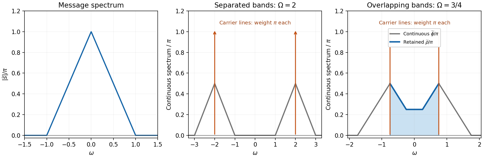
At $\Omega =3/4$, the two continuous triangles overlap near zero. Their amplitudes add, giving a central plateau. Explicitly, write $C(\omega )$ for the continuous part of $\tilde{\varphi }$:There are also the two carrier Dirac delta lines $\pi \delta (\omega \mp 3/4)$. The last panel of the preceding figure shows this spectrum and the retained central portion. The prescribed strict cutoff removes the carriers and keepsThe values of the ordinary function at individual endpoints do not affect its inverse transform. To handle the carrier lines, one must additionally assign zero filter gain to those lines, as the carrier-rejecting prescription indicates. A discontinuous mask has no canonical product with a Dirac delta at its discontinuity; a different physical boundary gain would leave a corresponding multiple of $\cos (3t/4)$.

The retained spectrum is real and even. Its inverse Fourier transform isIntegrating the linear factors yieldsThe removable value is $\boxed{\rho (0)=1/4}$, obtained either by expansion or by integrating $\tilde{\rho }/(2\pi )$. Because the carrier frequency is below the message bandwidth, this is Fourier filtering of overlapping amplitude-modulation sidebands; the usual picture of two isolated bands in single-sideband modulation does not apply without that qualification.

A direct way to avoid the singular transform of $1/t^2$ is to invert a triangular function. Evenness givesAt $t=0$ the limit is $1/2$, so there is no singularity in the original signal. ThusAlternatively, the hint uses the Hadamard finite-part reciprocal-power distribution, whose distributional Fourier transform is $\mathcal{F}[\mathrm{fp}(1/t^2)]=-\pi |\omega |$; combining its three translates gives $\pi (|\omega -1|+|\omega +1|-2|\omega |)/2$, the same triangle. Treating $1/t^2$ as an ordinary integrable function would be invalid.

The message spectrum has height $\pi$ at zero, vanishing at $\omega =\pm 1$. For $\Omega >1$, the modulated continuous spectrum consists of disjoint triangles of height $\pi /2$, centred at $\pm \Omega$, each with half-width one. In addition there is a Dirac delta carrier line of weight $\pi$ at each centre. These lines have specified area, not a finite height; arrows mark them schematically.

Use the Fourier transform conventionSince $\mathcal{F}[e^{i\Omega t}]=2\pi \delta (\omega -\Omega )$ in distribution theory, the carrier has transformThe modulation property of the Fourier transform translates the message spectrum to the two carrier frequencies. ThereforeThe first term represents the unmodulated carrier wave; the other terms are the amplitude modulation sidebands.

The left-hand value at the junction isThe right-hand value isThus the piecewise Green function solution is continuous, withIts derivative is continuous as well: both one-sided values equal $-\frac{1}{2}(1-e^{-\mu }{)}^2$. Only the second derivative jumps, consistently with the step in the forcing and the absence of a Dirac delta source.

Away from $x=\xi$, the homogeneous equation has solutions $e^x,e^{-x}$. A basis adapted to the two boundary conditions is $u(x)=\sinh x$ at the origin and $v(x)=e^{-x}$ at infinity. Their Wronskian is $u{v}^{\prime }-u^{\prime }v=-1$. The Green function must be continuous at $\xi$, while integration of $-G_{xx}+G=\delta (x-\xi )$ across the source givesThese conditions give the Dirichlet half-line Green function for minus d2 plus 1:where $x_{<}=\min (x,\xi )$ and $x_{>}=\max (x,\xi )$. The second term is the image that enforces $G(0,\xi )=0$; both terms decay as $x\to \infty$.

For the finite forcing interval, $y(x)={\int }_0^{\mu }G(x,\xi )d\xi$. When $x\le \mu$, split the integral at $\xi =x$:When $x\ge \mu$, the entire source interval lies to the left, giving the Dirichlet half-line response to uniform interval forcingThis solution is unique: a homogeneous difference satisfying the origin condition is proportional to $\sinh x$, which cannot decay at infinity unless its coefficient is zero.

With the specified ratios, the two factors in the modal amplitude become $\sin (n\pi /5)$ and $\sin (n\pi /14)$. Hence a normal mode is unexcited precisely when one of these factors is zero:That includes all multiples of five or fourteen, with multiples of seventy counted once. The mode $n=0$ is not a fixed-end string mode.

Assume the struck interval lies within the string, so $0\le \ell -a/2<\ell +a/2\le L$. The initially stationary straight string has $A_n=0$. Write its initial velocity as a Fourier sine series $g(x)={\sum }_n{g}_n\sin (k_{n}x)$. ThenThus $y(x,t)={\sum }_n(g_n/{\omega }_n)\sin ({\omega }_{n}t)\sin (k_{n}x)$. Immediately after the strike all the energy is kinetic energy:The orthogonality integral ${\int }_0^L\sin (k_{n}x)\sin (k_{m}x)dx=(L/2){\delta }_{nm}$ assigns energy $E_n=\rho L{g}_n^2/4$ to mode $n$. Since the ideal modes evolve independently, their total kinetic-plus-elastic energies remain constant. Therefore the modal energy of a localized velocity impulse on a string givesThe centre factor selects modes having significant motion at the impact location; the width factor accounts for cancellation across the finite hammer footprint. Parseval's identity ensures ${\sum }_{n\ge 1}{E}_n/E=1$. The velocity discontinuities are understood in the mean-square sense and do not alter the energy integrals.