
For a fixed pressure difference across two noncommunicating layers, an activated viscous polymer segment of length adds hydraulic resistance in series with the remaining fluid. The Darcy flux is the displayed expression when polymer raises dynamic viscosity by a factor . Tracking particle entry time determines activation and exit, while gives each displacement front. Preferentially occupying the more permeable layer shifts the relative inflow toward the other layer, but cannot increase that layer's absolute flux at fixed pressure. It can delay its breakthrough and leave original reservoir fluid flowing after the unmodified reservoir would be fully swept.
An aquifer is a permeable geological formation containing and transmitting groundwater. A confined aquifer lies beneath a confining layer; an unconfined aquifer instead has a free water table.
The logistic growth equation applies the logistic differential equation to population dynamics. For positive growth rate and carrying capacity , an initial condition gives , where . Its per-capita growth falls linearly with abundance, and a trajectory starting below reaches an inflection point when . The exact solutions of a differential equation and their diagrams are developed under logistic differential equation. A translated and scaled logistic function has the same form. In nonlinear regression for biological size, an analogous saturation curve need not imply that circumference itself obeys a mechanistic population law.
Two populations grow at the same per-capita rate and each loses members at a rate proportional to their product. On the invariant diagonal , the logistic differential equation gives for and positive rates. The positive symmetric equilibrium is stable along that diagonal but unstable transversely: , while the Jacobian matrix has eigenvalues . Thus an exactly symmetric deterministic solution can relax toward coexistence while a small imbalance grows. A corresponding density-dependent Markov jump process has a controlled fluid limit on each fixed finite interval, rather than uniform control for all time.
The Nicholson-Bailey model describes seasonal host-parasitoid interaction. Hosts surviving random attacks reproduce, while parasitoid offspring are proportional to attacked hosts. For , its positive equilibrium is , . Counting attacked rather than surviving hosts makes its predator reproduction law different from the annual pulse-breeding predator-prey model.
A carrying capacity is an abundance scale at which a specified environment's net population growth vanishes. In the logistic growth equation, positive unharvested populations approach . It depends on the species, resources and environment rather than being an immutable universal population limit.
The useful distinction is between a growth rate and a sustainable abundance. In a logistic differential equation, controls how quickly a population responds, while the carrying capacity sets the positive equilibrium point. Increasing with fixed accelerates approach without raising that equilibrium. Increasing changes the destination. The logistic differential equation diagrams show populations approaching the same carrying capacity from below and above.
In ecological use, the carrying capacity describes what a particular environment can support under specified conditions. Nutrient supply, available space, and accumulated waste can change those conditions; it is not a permanent property of a species alone. A population temporarily above a carrying capacity is possible. In the simplest constant- logistic growth equation, its net growth becomes negative; real population dynamics can include delays, seasonal variation, and changing resources that the basic mathematical model omits. [ref]
https://openstax.org/books/biology-2e/pages/45-3-environmental-limits-to-population-growth. Clark, Douglas and Choi, Biology 2e, §45.3: carrying capacity and environmental limitations
.Cellulose is a polysaccharide of glucose units whose chains form strong assemblies in plant cell walls. It illustrates a structural role for carbohydrates. See Alberts et al., Molecular Biology of the Cell: the plant cell wall.
A polynomial identity is equality of formal polynomials: every corresponding polynomial coefficient agrees. For example, holds in the polynomial ring over every commutative ring. Polynomial evaluation preserves such an identity, so it gives an equality of values at every allowed substitution.
The converse requires a hypothesis on the coefficient field. Over an infinite field, a polynomial that vanishes at every point is zero: use the Lagrange root bound over a field in one variable, and induction on the number of variables. Over the finite field , the nonzero formal polynomial induces the zero polynomial function. Thus equality of polynomial functions on a finite domain need not be a formal polynomial identity. Coefficient comparison, as used with the binomial theorem, concerns formal polynomial identities.
A quadratic polynomial in one variable over a field has polynomial degree two and the displayed form. Its roots of a polynomial satisfy a quadratic equation. The polynomial and its associated polynomial function are distinct objects: over a finite field, different polynomials can define the same function.
If polynomials of degree at most converge at distinct points, their coefficients converge, by invertibility of the Vandermonde matrix. Their limit is a polynomial of degree at most , and convergence is uniform on every compact subset of . Under convergence on compact sets, Rouché's theorem further locates a unique nearby zero for each simple root of the limit, for all sufficiently large indices. Finite initial polynomials need not have any root.
Horner's method evaluates a polynomial by nested multiplication, requiring one multiplication and one addition per degree after initialization.
For , start with and compute for . The final value is . Equivalently,This reorganization reuses intermediate results, avoiding separate computation of every power. A dense degree- polynomial takes multiplications and coefficient additions after reading its leading coefficient; special zero coefficients may permit further simplifications.
For our cubic, the coefficient list in descending order is . The zero is important: it occupies the missing term's position. At , the accumulated values areAt , the same operations give , confirming .
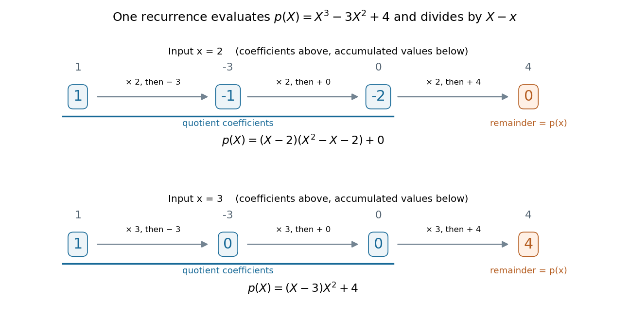
The same nested arithmetic evaluates a polynomial and produces the coefficients for division by a linear factor
. Details. 
The intermediate values do more than evaluate. They are the coefficients of the polynomial quotient in polynomial division by , with the final value as the polynomial remainder. At , the first three values give , soAt , they give , so . This links an efficient numerical calculation with the exact factor theorem.
William George Horner's 1819 paper concerns solving numerical equations by successive approximation. The Royal Society archive records the manuscript and its reading on 1 July 1819; it provides a historical reference for the method's name. [ref]
// Target: geometry-and-topology.bigb
The reciprocal polynomial reverses the coefficients of a polynomial with nonzero constant term. For a binary cyclic code with generator and canonical check polynomial , the reciprocal generates the dual of a cyclic code.
// Target: algebra.bigb
The Hasse derivatives of a polynomial are the coefficients in . A point has multiplicity at least exactly when for . Unlike iterated formal derivatives divided by factorials, this definition works in positive characteristic, where factorials can vanish. For example, in characteristic two has zero first formal derivative but nonzero second Hasse derivative.
// Target: coding-theory.bigb
Over a field of characteristic , additive polynomials are sums of -power monomials, . They act linearly over the prime field. The identity follows from the Frobenius endomorphism; the converse follows by comparing mixed binomial coefficients. Their zero sets are additive groups, and a nonzero linear coefficient makes all roots simple.
An indeterminate is a formal symbol used to construct a polynomial. Choosing an input later defines a polynomial function; the symbol itself is not a fixed member of the coefficient ring.
Polynomial evaluation replaces the indeterminate of a polynomial by an input value. For a fixed scalar , the rule is a linear functional on a vector space of polynomials, because evaluating a linear combination gives the same linear combination of the values. For , evaluation at zero gives one and evaluation at two gives seventeen. Polynomial interpolation uses these measurements to reconstruct a polynomial subject to a polynomial degree bound.
A polynomial factorization expresses a polynomial as a product of other polynomials. The allowed coefficients matter: has no nonconstant factorization over the rational numbers, but factors as over the real numbers. Difference of squares gives over any commutative ring.
An angiosperm pollen grain is a small male gametophyte, not itself a seed or a single gamete. Its tube-forming biological cell supports delivery of sperm.[ref]
Observing the growth of pollen tubes (Practical Biology). Teaching notes: pollen grain and tube as male gametophyte
For , , use entry and exit . If , , integration gives . A smooth global return has . If , its derivative vanishes as , and a small yields an attracting fixed point. If , the passage is . For small parameters the resulting global return is strongly contracting, with an attracting fixed point near on either side of zero.
There are unlisted articles, also show them or only show them.