
A dielectric is a material in which an electric field produces electric polarization while transport of electric charge is sufficiently small for the intended use. An insulating solid in a capacitor is an example; real dielectrics can still have dielectric loss and nonzero electrical conductivity.
The important distinction is between rearranging bound electric charge and transporting mobile charge carriers through the specimen. Bound electric charges can move a little within a chemical atom or molecule, or an existing electric dipole can turn. Their averaged electric dipole moments produce electric polarization even if there is negligible steady electric current between the electrodes. A changing electric polarization does give a bound current; the absence of steady conduction does not mean that the material is electrically unresponsive.[ref]
For uniform electric polarization in a rectangular slab, polarization density gives zero bound volume charge density in the interior and opposite bound surface charge densities on the left and right faces. The electric charge has been redistributed, not created. More generally, the divergence theorem makes the cancellation explicit:Here is the outward normal vector on the material boundary. This accounts for both bound volume charge density and bound surface charge density; omitting either can falsely suggest that an initially neutral dielectric acquired net electric charge.
An electrical insulator between capacitor plates supports a useful combination: appreciable electric polarization, little leakage electric current, and tolerance of the intended electric field. This lets a small parallel-plate capacitor store separated electric charge and recoverable capacitor energy. The comparison in dielectric capacitor response explains why specifying fixed electric charge or fixed electric potential difference changes the answer. High relative permittivity alone does not establish good insulation or a large usable energy density; dielectric loss and dielectric breakdown matter as well.
Thawing permafrost makes previously frozen organic matter available for decomposition, releasing carbon dioxide and, in waterlogged oxygen-poor conditions, methane. These greenhouse gases amplify warming, which can cause further thaw. The amount reaching the atmosphere depends on decomposition, transport and oxidation; this feedback does not imply an inevitable abrupt release of an entire carbon reservoir.
A periodic table period is a horizontal row of the periodic table, read in increasing atomic number. Periodic table period 2 runs from lithium, , to neon, : chemical elements. In these neutral ground states, the second electron shell gains electrons while the first retains two.
A periodic group is a vertical column of the periodic table. For example, fluorine and chlorine are in periodic group 17, with seven valence electrons in each neutral ground state chemical atom. A shared outer electron configuration supports similarities in chemical reactions, rather than equality of every property.
A periodic orbit of a differentiable interval map is superstable when its periodic-orbit multiplier vanishes. A cycle passing through a critical point has zero multiplier because the derivative product includes . For the nonconstant quadratic family , a superstable cycle satisfies and does not have a smaller critical period.
// Target: dynamical-systems.bigb
Somatostatin is a peptide hormone that inhibits secretion in several endocrine and digestive contexts. Pancreatic delta cells release it locally, where it can restrain insulin and glucagon secretion. Its effects depend on receptor subtype and target cell rather than a universal suppression of all cellular activity. Processing of a common precursor generates biologically active peptide forms of different lengths. [ref]
UniProtKB by the UniProt Consortium. P61278, Function, Catalytic activity and Subunit structure
With Hardy-Weinberg equilibrium, let count copies of the risk allele. The penetrance must lie in for every possible genotype. Writing and gives and .
For a binary disease trait with genotype , the genetic variance of penetrance is the between-genotype term in the law of total variance. The averaged within-genotype term is . Under multiplicative diallelic penetrance, the genetic term is . This decomposition attributes variance to the modeled locus, not automatically to all hereditary causes.
Pedigree peeling eliminates latent genotypes by moving sums inside products whenever the other factors do not depend on the eliminated genotype. For one parent genotype and one child genotype , the likelihood becomesThe inner bracket is the child's message to its parent. With two states each, it needs four multiplications and two additions; multiplying the two parent weights and messages needs four more multiplications and the final sum one addition. The unrearranged four terms instead use twelve multiplications. Larger pedigrees use the same variable-elimination identity, with additional handling of pedigree loops.
Assign one genotype random variable to each person in a pedigree. Independent founders in a pedigree carry population genotype laws, and each other genotype has its conditional distribution given its two parents from Mendelian segregation. The ancestry directed acyclic graph is a Bayesian network for the joint genotype law. Its moral graph contains each parent-child edge and each coparent edge. Each founder factor and each child-with-parents factor belongs to a clique, giving an undirected graphical representation. The graph is an independence representation; equality with the minimal conditional independence graph needs additional faithfulness assumptions, particularly because inheritance can produce zero probabilities.
An unphased multilocus genotype can have several pairs of haplotypes. Its pedigree likelihood must average over these possible phases with prior weights , rather than maximize over phases after observing the offspring. Under linkage disequilibrium, the weights need not be equal. They can be obtained by conditioning biological population haplotype frequencies on the observed parental genotype; different choices of what is conditioned on change only parameter-independent factors when those frequencies are held fixed.
A Pauling bond-energy excess subtracts a chosen like-atom baseline from the unlike-atom bond-dissociation energy. For an unequal-input arithmetic example, stipulate , and , all with one dissociation convention. The arithmetic mean baseline and excess areThe arithmetic-baseline Pauling scale model therefore gives . The bond-dissociation energy is not itself the excess: subtracting the baseline is essential. All three numbers are stipulated, not experimental values for named chemical elements.
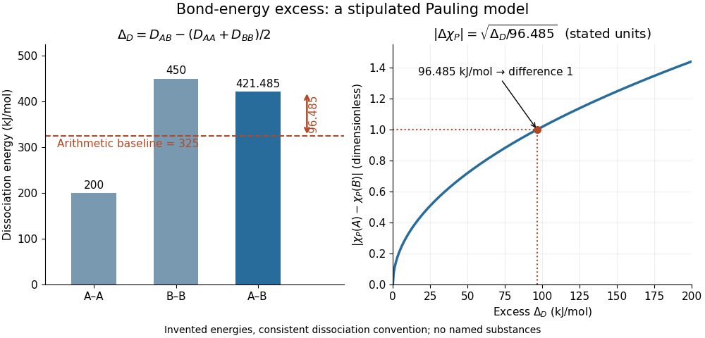
Constructing a Pauling bond-energy excess from stipulated bond-dissociation energies and converting it to a dimensionless electronegativity difference
. Details. 
Changing the baseline changes the model. For the same stipulated inputs, a geometric mean baseline would be , yielding an excess of and a difference of approximately . It is a different construction, even though both start from the same bond-dissociation energies. State which baseline is used before comparing electronegativity differences.
The arithmetic-baseline Pauling scale also has a useful inverse: a difference of corresponds to an excess of , and a difference of corresponds to . Doubling the electronegativity difference quadruples the modeled excess. Interchanging the endpoint labels changes neither quantity; the square root alone cannot choose the direction of bond polarization.
In The Nature of the Chemical Bond. IV. The Energy of Single Bonds and the Relative Electronegativity of Atoms (printed pp. 3576–3578, Table II and equation (1)), Linus Pauling organized excess energies for chemical bonds into an approximately additive map of their square roots. He also identified a limitation: his H–F map separation of predicted an excess of , exceeding his table's value by . Those are historical values and a historical model discrepancy, not modern recommended inputs.[ref]
The Nature of the Chemical Bond. IV. The Energy of Single Bonds and the Relative Electronegativity of Atoms by Linus Pauling. printed pp. 3576–3578, Table II, equation (1), and paragraph beginning “These coördinates”
A traceless Hermitian matrix in a Hilbert-Schmidt inner product orthonormal basis of the real vector space of traceless Hermitian -by- matrices. One choice uses symmetric and imaginary antisymmetric off-diagonal matrix units, normalized by , and traceless diagonal generators. Together with they form an orthonormal basis of all Hermitian matrices. The coordinates give the Generalized Bloch representation.
For with , take . The spin-down transverse Hamiltonian at momentum label is proportional to , where . It is nonnegative, and gives the displayed zero mode. Since , its exponent has a negative quadratic upper bound at both infinities, proving square integrability for every . The continuously varying momentum label supplies an infinitely degenerate zero-energy space.
The complement of finitely many lines in is path-connected, and any two points can be joined by two line segments. For endpoints outside the lines, exclude the finitely many affine planes through each endpoint and each removed line. Choose a bend point outside all those planes. If either segment met a removed line, the bend point would lie in its associated excluded plane, a contradiction.
The union of with horizontal segments for rational is path-connected. Each point lies either on the vertical spine or on a segment meeting it. A path travels horizontally to the spine, vertically along it, and horizontally to its destination. This contrasts with disconnected rational-slope rays whose common origin has been excluded.
The map for , , is continuous on , since . Its image is the displayed spiral together with its endpoint. The image is compact and path-connected: between images of the explicit path is .
The comoving particle horizon is the particle horizon expressed in comoving coordinates, assuming a finite initial cosmic-time boundary at zero. In a spatially flat FLRW metric, it is the distance a photon could have travelled since that boundary. The corresponding proper distance in cosmology at time is . It differs from the future-directed cosmological event horizon and from the instantaneous comoving Hubble radius.
There are unlisted articles, also show them or only show them.