
An SH2 domain is a protein domain that recognizes a phosphotyrosine residue together with surrounding sequence features. This selective binding recruits a protein to a modified receptor or docking protein; it does not itself imply catalysis.[ref]
Signaling through Enzyme-Linked Cell-Surface Receptors. “Phosphorylated Tyrosines Serve as Docking Sites For Proteins With SH2 Domains”, Figure 15-53
The critical path method calculates an earliest schedule, a latest schedule for a chosen finish time, and each activity's task float. A critical path is a start-to-finish graph path whose total duration is greatest. There can be several such graph paths, and every one constrains completion. In the six-activity project scheduling example, the critical graph path is A-C-D-F, of duration .
Add a zero-duration source before every initial activity and a zero-duration sink after every terminal activity. Give each edge weight , including zero weight on edges leaving . This produces a weighted graph in which a graph path's weight counts every activity on it exactly once. The possible source-to-sink graph paths in our example, omitting the dummy endpoints, are A-B-D-F with weight 8, A-C-D-F with weight 10, and E-F with weight 4.
Every feasible schedule must accommodate each of these sequential chains. Consequently,This bound applies to all source-to-sink graph paths, not just the one we happen to inspect. The critical path method attains the bound by setting each activity's earliest start to the maximum of its predecessors' earliest finish times:Evaluate this recurrence in a topological order, obtained by topological sorting. Each satisfies every incoming optimization constraint, so these times form a feasible solution. The same recurrence calculates the greatest weight of a graph path from to ; hence the feasible finish matches the lower bound. This is dynamic programming on a directed acyclic graph, rather than an enumeration of all graph paths. See Paul Johnson, Scheduling and longest paths, longest-path algorithm. The linear programming formulation and its certificate are developed in project scheduling duality and unit-flow certificate for project duration.
For our project scheduling example, , , and the two merges giveF finishes at 10. All six activities are completed, even though E is absent from the critical graph path. Recording which predecessor attains each maximum lets us trace a critical graph path backward from the sink; retaining tied choices exposes multiple critical graph paths.
Now fix the project start at zero and the finish at . The latest starts come from a backward pass in reverse topological order:Every activity must finish by the earliest of its successors' latest starts, explaining the minimum here. This gives , , , , , and . These latest times themselves form a feasible solution finishing at 10. The backward calculation depends on the chosen finish time; a later deadline would give different latest times and task floats. The forward and backward passes are described in Olivier de Weck, MIT ESD.36 Lecture 2, slides 22–29.
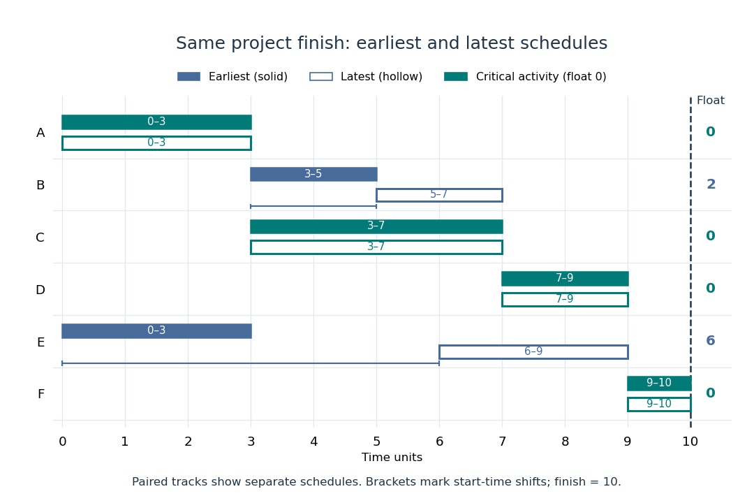
Earliest solid and latest hollow activity bars for the critical path method, with task floats of 2 for B and 6 for E
. Details. 
Changing a duration can change which graph paths are critical. If B's duration becomes 4, A-B-D-F and A-C-D-F both take 10: there are two critical graph paths. Shortening C alone then cannot reduce the finish time, because the chain through B still takes 10. If B's duration instead becomes 5, the earliest starts of D and F become 8 and 10, and the finish becomes 11. A-B-D-F is now the unique critical graph path; C has task float 1 relative to that new optimal finish. These calculations show why the critical path method is useful for understanding where a duration change matters, even in a project containing many parallel activities.
The syntactic priority that resolves grouping when different operators occur together without parentheses. It determines the abstract syntax tree shape before evaluation.
An arbitrary product of compact spaces is compact in the product topology. The theorem is equivalent to the axiom of choice.
The diagonal map sends to . It is an embedding of a topological space onto its diagonal subset, because either coordinate projection is its inverse on the image. For a closed oriented manifold, that subset has a fundamental class, whose Poincare dual is the cohomology class of the diagonal.
A function on a Cartesian product is a cylinder function if it depends on only finitely many coordinates. With finite discrete coordinate spaces it is a continuous function in the product topology. These functions determine finite-dimensional laws and provide a natural domain for local generators of interacting particle systems.
For a topological space and topological spaces , a function is continuous into the product topology exactly when every coordinate function is continuous.[ref]
18.901, Fall 2024 lecture notes. Lecture 5, Proposition 5.3.2, printed page 21: continuity into a product is equivalent to continuity of all component functions
Proof outline: one direction uses function composition with the continuous projection maps. For the other, the preimage of a basic cylinder set isa finite set intersection of open sets in . This gives continuity on every basic test. It explains, for example, why from the real line to is continuous in the product topology: each coordinate is a polynomial function. The general coordinate criterion fails for the box topology, where infinitely many preimages can be required at once. For example, has continuous coordinate functions, but the preimage of the box is , which is not an open set in the real line.
The box topology on has a basis of a topology consisting of all Cartesian products with every an open set in ; infinitely many coordinates may be restricted. It contains the product topology and agrees with it for finite .[ref]
18.901, Fall 2024 lecture notes. Lecture 12, Exercise 12.1.2(1)-(2), printed page 43: box basis, comparison with the product topology, and finite-factor equality
For copies of the usual real line, the box topology is strictly finer when . The box is not an open set in the product topology: a basic cylinder set containing zero leaves some coordinate unrestricted, so it contains . This is a construction for every finite coordinate set, not evidence from testing a finite prefix.
For arbitrary topological spaces , an index set , a sequence , and a point in that Cartesian product, convergence in a product space to in the product topology is equivalent to coordinatewise convergence in every factor. No countability or Hausdorff assumption on the factors is needed. For a product space of copies of the real line, regarding each point as a function identifies this with pointwise convergence.
Proof outline: the forward implication follows because each projection map is continuous. Conversely, given a basic neighborhood of , each of its finitely many coordinate tests holds for all . Taking makes all tests hold simultaneously; if is empty, any threshold works. This proves eventual membership in every neighborhood, rather than only in a sampled collection of cylinders. The same equivalence holds for nets: a directed set supplies a common upper bound for finitely many thresholds. Sequences alone need not characterize the whole topology of an arbitrary product space.
For a finite set and open sets for , the setsform a basis of a topology for the product topology. The empty set intersection is . Each basic open set is a cylinder set; all coordinates outside are free. Arbitrary open sets are unions of these basic tests and need not themselves depend on one fixed finite collection of coordinates.[ref]
Point-Set Topology, Chapter 2: Continuous functions. Proposition 2.2.1, Definition 2.2.2 and Remark 2.2.8: finite-coordinate basis and general open subsets
Why finitely many? Any topology making the projection maps continuous must contain their preimages of open sets, and hence finite set intersections of those preimages. Taking arbitrary unions supplies exactly the product topology. Intersecting two basic cylinder sets still restricts only the finite union of their coordinate sets.
Thinning removes points from a point process according to a retention rule. independent retention with probability changes the intensity measure to . For a Poisson point process, the retained and removed point processes are independent Poisson processes.
Let be probability measures on the real line with characteristic functions . Lévy's continuity theorem says that if converges for every real to a function continuous at zero, then is the characteristic function of a unique probability measure and converges weakly to . Conversely, weak convergence implies pointwise convergence of characteristic functions to the characteristic function of the limit.
The converse follows immediately by testing against the bounded continuous functions . The difficult direction uses continuity at zero to control probability escaping to infinity, and the uniqueness of characteristic functions to identify every subsequential limit. The theorem turns convergence of probability laws into convergence of ordinary functions, which is especially useful when independence makes characteristic functions multiply.
Continuity at zero is essential. For , tends to zero for every nonzero but remains one at . This discontinuous limit is not a characteristic function, and the distributions have no weak probability limit: their mass in every fixed bounded interval tends to zero.
A standard score expresses an outcome as a signed number of standard deviations from a mean , assuming . It is a dimensionless quantity. For a random variable with finite positive variance , has mean zero and variance one; it has a standard normal distribution when has a normal distribution, but centering and scaling alone do not make other probability distributions normal. [ref]
https://ocw.mit.edu/courses/18-05-introduction-to-probability-and-statistics-spring-2022/mit18_05_s22_class06-prep-b.pdf. MIT 18.05, Reading 6b, §5.1: standardization
.Pairwise independent events describe a subtle kind of uncertainty: learning that one event occurred leaves each other event's probability unchanged, yet learning that two occurred can reveal a third completely. Checking every pair therefore answers a weaker question than checking the whole collection. The parity construction of pairwise independent bits makes this distinction visible with just four equally likely outcomes.
A family of events is pairwise independent whenIf , this is equivalent to the conditional probability identity . The product definition also handles events of probability zero. Independent events, meaning mutually independent events, require the same product rule for every finite subfamily, including triples. For three events, the three pair equations and the triple equation are four separate requirements. [ref]
https://www.randomservices.org/random/prob/Independence.html. Kyle Siegrist, Random Services: independence of two events and general independence of events
.For a worked example, take independent fair bits : the sample space is with probability per outcome. Set , , and , using exclusive or, which is one precisely when its inputs differ. The events , , and each contain two outcomes. Their pair intersections areThus each event has probability and each pair intersection has probability : these are pairwise independent events. But forces , soThe three are not independent events. This is the complementary-third-event version of the two-toss example in Tsitsiklis and Jaillet, MIT Introduction to Probability, Lecture 3, slides 7–8.
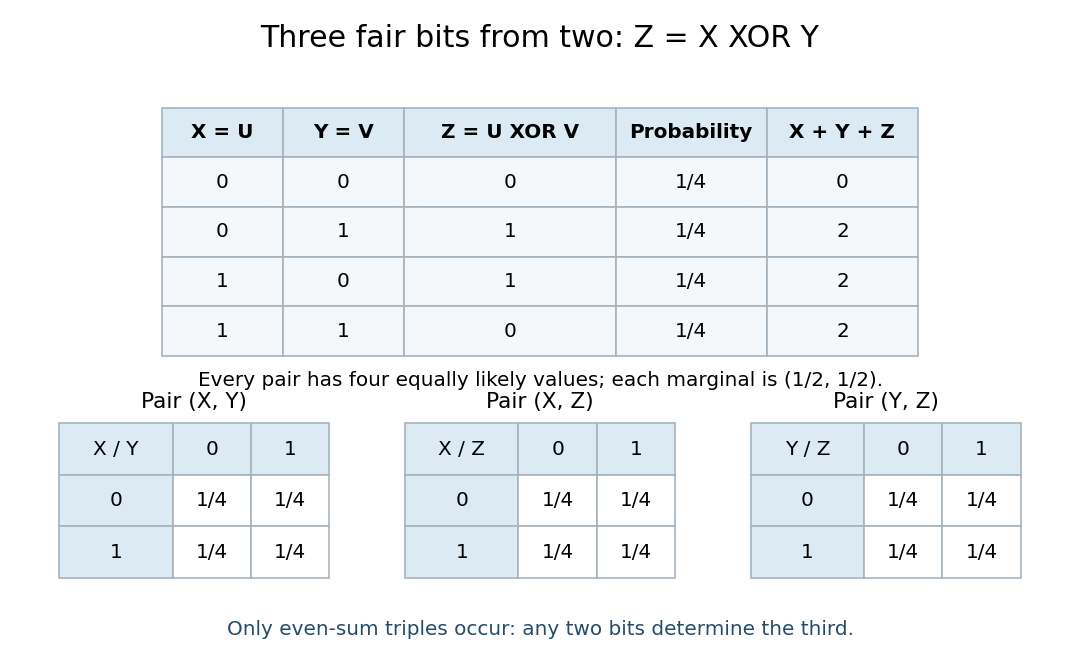

Another useful diagnostic preserves a special common-intersection case. Suppose three events have common probability and every pair and triple intersect in the same event, of probability . Pairwise independence requires , while mutual independence additionally requires . Both hold only for or . For a concrete nontrivial instance, assign probability to each of four outcomes, let all three events contain the first outcome, and give each event one different additional outcome. Then and : the pair equations hold, while the triple equation fails. Unlike the exclusive or example above, this triple intersection is nonempty.
The probability that independent uniformly oriented open hemispheres cover a sphere is the displayed quantity. Coverage fails exactly when their normals lie in a closed hemisphere. With probability one, no three normals are coplanar and no pair is antipodal; a closed hemisphere containing the normals can then be perturbed into an open one. Condition on the unoriented axes of the normals. Their orientation signs remain independent fair bits, and the regions of a general-position great-circle arrangement realize exactly of the possible sign vectors. Each such vector corresponds to normals that fit into one open hemisphere, proving the complementary probability. The argument counts equiprobable orientation choices, not equal-area regions.
For independent lengths with the uniform distribution on , the probability of forming a nondegenerate polygon is . The necessary and sufficient condition is that every length is less than the sum of the others. The failure events are disjoint except on sets of probability zero. The sum of lengths has probability density function on , by repeated convolution of probability densities. A specified rod is too long with probability ; summing over the rods proves the formula. For three and four rods the probabilities are and .
Different precise measures on random chords give different probabilities; the phrase “random chord” does not select a unique probability distribution. In a circle of radius , a chord exceeds the side of an inscribed equilateral triangle exactly when its midpoint distance from the center is below . Uniform midpoint area gives probability , independent uniform endpoints give , and uniform midpoint distance gives . The difference is in the sampling laws, not a contradiction in probability theory.
For water initially at rest at depth on one side of a dam and a dry bed on the other, a channel with has . The centered rarefaction wave has and . Thus and within . The reservoir remains undisturbed to the left and the bed dry to the right. This is an outer shallow-water approximation before finite-reservoir boundary signals return.
In a prismatic triangular channel with wetted area proportional to , the Riemann invariants are , with . Releasing water initially at rest into a dry channel produces a rarefaction wave with and . Hence , and the displayed depth profile for . The dry front advances at before finite-reservoir or varying-channel effects become important.
A channel with width has wetted area . Its inviscid shallow water equations have characteristic speeds and the displayed Riemann invariants. Releasing a reservoir of depth at rest into a dry channel gives a left-family rarefaction wave: , , between and , where . This width law differs from a geometrically parabolic trough, whose width is proportional to .
There are unlisted articles, also show them or only show them.