
Spectral luminous efficacy converts radiant flux at one wavelength to luminous flux. The candela convention fixes exactly at , not at an exactly specified wavelength of . [ref]
In vacuum, that frequency corresponds to , using the speed of light. In standard air it is approximately , close to the maximum of the photopic luminous efficiency function. Thus is slightly larger than ; using in ordinary calculations is a rounded convention. The exact anchor is . [ref]
Scotopic vision is vision at low illumination dominated by rod cells. It provides high sensitivity to weak light but little of the color discrimination associated with cone cells. Consequently equal radiant powers at different wavelengths need not appear equally bright, and brightness comparisons change with illumination level.
A simple observation compares colored patches as illumination is reduced after adaptation: their relative brightness can change even though the illuminating optical spectrum is held approximately fixed. Controlled measurements must allow adaptation and avoid stray illumination. A photopic luminous efficiency function is appropriate to a different viewing regime and cannot be used indiscriminately for scotopic vision.
Photopic vision means vision under light-adapted conditions. Standard photometry here uses the photopic luminous efficiency function; scotopic vision uses a different weighting for dark-adapted conditions. The response function and adaptation conditions must be stated when comparing luminous fluxes.[ref]
Mise en pratique for the definition of the candela and associated derived units for photometric and radiometric quantities in the SI. §3.1, printed p. 3: photopic and scotopic luminous efficiency functions
The photopic luminous efficiency function is dimensionless and describes standardized relative sensitivity for photopic vision. It is normalized to and tabulated over –. The wavelength coordinate is in standard air, rather than vacuum; changing coordinates requires converting the spectral radiant flux density as well. The official prescription uses linear interpolation between the specified 1 nm entries.[ref]
Mise en pratique for the definition of the candela and associated derived units for photometric and radiometric quantities in the SI. §3.1, printed pp. 2–3: wavelength convention, normalized functions and interpolation
Write for the standard-air wavelength at . With spectral radiant flux in and in nanometres, the luminous flux isThe integral has units of watts, and converts them to lumens. For radiation at a single wavelength with total radiant flux , this reduces to . For a sufficiently narrow finite band, this is an approximation requiring nearly constant across the band.[ref]
For isotropic specific intensity , absorption cross-section , and threshold frequency , the photoionization rate per target atom isFor a directed incident flux, replace by its spectral flux density. The factor converts energy flux into photon flux. This rate alone does not imply photoionization equilibrium.
A molecular nitrogen experiment used a pulsed nozzle and two skimmers. A tube raised the rotational temperature. Opposed vacuum-ultraviolet laser pulses excited selected molecular levels and, about later, selectively ionized excited nitrogen fragments. A microchannel plate detector, phosphor screen and camera recorded radii.[ref]
Accurate measurements of the bond dissociation energies of 14N2, 14N15N and 15N2 by Liya Lu and others. Lu, Jiang and Gao, §2, printed manuscript pp. 2–3: nozzle, tube, pump/probe and imaging readout
The measured squared radii were fitted against molecular excitation energies, referenced to the parent ground state:The intercept at zero radius gave the excited-product threshold; the fitted slope absorbed the detector scale. A wavemeter monitored the excitation source; scanning the probe covered the recoil Doppler shift. Subtracting the atomic excitation energies converted the intercept to ground-product .[ref]
Accurate measurements of the bond dissociation energies of 14N2, 14N15N and 15N2 by Liya Lu and others. §1: image-radius equation; §2: wavemeter and probe scan; §3 and Figure 4: fits; §4: atomic excitation correction
An apertured grounded plate and detector timing rejected faster competing channels. Selecting fragment electronic states distinguished nearby thresholds. Agreement of across isotopes after zero-point energy correction tested consistency. The method still requires correctly assigned levels, adequate near-threshold signal and stable imaging; a signal drop alone can reflect another channel or a barrier.[ref]
Accurate measurements of the bond dissociation energies of 14N2, 14N15N and 15N2 by Liya Lu and others. §2: shielding plate and timing; §3: state-selected channels; §4 and Table 2: isotope consistency and limitations
This measurement determines a state-resolved ground-state dissociation energy. Obtaining a finite-temperature bond-dissociation enthalpy requires the thermal increments above; obtaining a bond potential-well depth requires the zero-point energy correction. The three quantities describe different starting conditions for the same specified separation.
Sphingomyelin is a phospholipid whose backbone is based on sphingosine, rather than glycerol. One long hydrocarbon region belongs to that backbone and another comes from an attached fatty acid. It is a counterexample to defining every phospholipid by the illustrated glycerol scaffold. See Cooper, The Cell: the molecular composition of cells.
Glycerophospholipids are phospholipids built on a glycerol-phosphate scaffold. The illustrated two-acyl group form is common, but the subclass also includes other substitutions and one-chain derivatives. See IUPAC–IUB lipid nomenclature, Lip-2.2 and Lip-2.6.
For unit-mass motion in , the mechanical energy is . The origin is a center equilibrium, and is a saddle equilibrium. Energies have trapped periodic orbits around the origin as well as a separate escaping component to the right. The barrier energy has a homoclinic orbit returning to the saddle after a turn at , plus two saddle branches on . Above the barrier, particles traverse the well and eventually escape to the right.
For , , the energy satisfies . At , its compact level sets give two families of closed periodic orbits around and an outer family around both; is a figure-eight homoclinic orbit pair through the saddle point at the origin. The two minima of are center equilibria for zero damping, stable foci for small negative , and unstable foci for small positive . For , strict monotonicity along nonconstant solutions excludes periodic orbits and homoclinic orbits.
For , the difference vanishes on and multiplies by . Its operator norm is therefore . Choosing the nearest angle on the grid , with circular distance, gives and a uniform bound of this size on the output-state norm error. This bound concerns state vectors, not an asserted equality with measurement-probability error.
Wick theorem expresses a time-ordered product of free fields as its normal-ordered product plus the sum over every possible contraction. It turns the Dyson series into Feynman diagrams.
A permutation with no fixed points. Applying the inclusion-exclusion principle to the events that each element is fixed gives . Therefore , and the alternating-series remainder is at most .
// Destination: foundations-of-mathematics.bigb
In a uniformly random permutation of objects, the cycle containing one specified object has a uniform length on . For length , choose the other objects, arrange their order around the tagged object, and permute all remaining objects. The count is , independent of . Its mean is , while the mean number of other elements in that cycle is .
A uniform random permutation of distinct objects gives each of the permutations the same probability. Restricting the order to any fixed subset gives a uniform ordering on that subset. Relative ranks encode such a permutation bijectively by independent choices of an insertion position.
A finitely supported permutation fixes every element outside some finite subset. The finitely supported permutations of are the union of the finite symmetric groups acting on , and hence form a countable set. All permutations of form an uncountable set: independently swapping or fixing each pair injects the power set of into this larger set.
A cyclic permutation, also called a permutation cycle, sends distinct elements and fixes every element outside this list. Its notation is . For example, is the permutation with image list : all four labels lie on one directed loop. In contrast,has two separate loops, exchanging with and with . It is a permutation composed of two transpositions, rather than a single cyclic permutation.
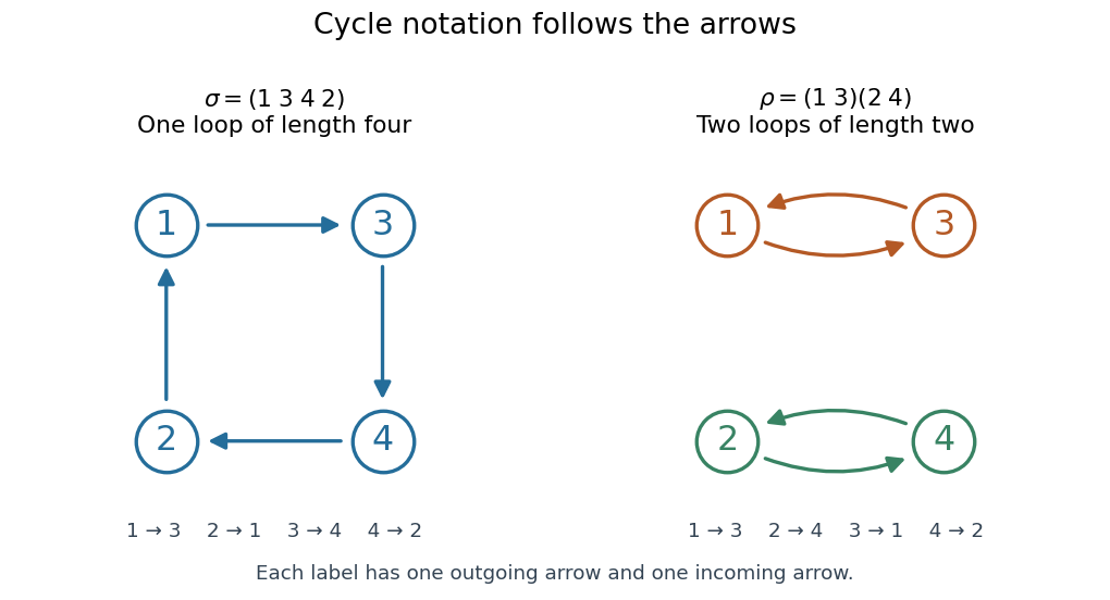
Two permutations on four labels: one cyclic permutation and two disjoint permutation cycles , with arrows showing every image
. Details. 
Starting at a different point of the same loop changes the written list but preserves the cyclic permutation: . Reversing the direction generally changes the permutation; it gives the inverse function, here . A transposition is a cyclic permutation of length two; a one-element permutation cycle records a fixed point. In a cycle decomposition of a permutation, one-element permutation cycles are usually omitted, with the underlying set understood.
The beauty of this representation is that repeated rearrangements become motion around independent loops. Applying four times returns every label to its start, while applying twice already does so. Disjoint permutation cycles commute under function composition, since each moves only labels the others fix. On labels, there are cyclic permutations whose single loop contains every label: fix as the first written entry and order the other labels freely, giving a factorial. This is also the count of cyclic orderings; choosing a starting position would otherwise count each loop times. Rotations are identified here, while reversing direction is allowed to give a different cyclic ordering.
Proof outline for decomposition. Starting at any label in a finite set, repeatedly apply the permutation. The pigeonhole principle forces a repeated label. If the first repetition were at a label other than the starting one, its two predecessors would be different labels with the same image, contradicting the injective function property. This produces a permutation cycle returning to the start. Start again at a label not yet visited; the new permutation cycle cannot meet an earlier one, since the bijection gives every label a unique predecessor. Continue until every label belongs to a loop. The resulting cycle decomposition of a permutation is unique up to the order of the disjoint permutation cycles and the starting point written in each one. [ref]
https://math.mit.edu/~fgotti/docs/Courses/C.%20Combinatorial%20Analysis/11.%20Permutations%20I/Permutations%20I.pdf. Felix Gotti, MIT 18.211, lecture 11, definitions 1–2 and the preceding argument
The motivating observation is that inserting an insulating material between fixed capacitor plates increases its capacitance. [ref]
https://www.feynmanlectures.caltech.edu/II_10.html#Ch10-S1. Feynman, Leighton and Sands, II.10–1, opening paragraphs: observed increase in capacitance with an inserted insulator
. To investigate this response, use two flat parallel metal electrodes with measured overlapping area and separation , a uniform specimen filling the gap, and an instrument that measures electrical impedance. Record the capacitance with and without the specimen at the same small applied electric potential difference, frequency and temperature, after capacitance measurement calibration. An increase in corrected capacitance indicates a larger permittivity, provided the geometry is unchanged. A guard electrode reduces the contribution of the fringing field of a capacitor. [ref].For negligible dielectric loss in the parallel-plate capacitor approximation,An air reference approximates ; it is not an exact vacuum reference. For the following synthetic example, stipulate , and the rounded vacuum permittivity . Then in this model, and relative permittivity four gives . A residual parallel capacitance of would make an uncorrected sample/reference ratio , rather than four. This additive error does not cancel in a ratio.
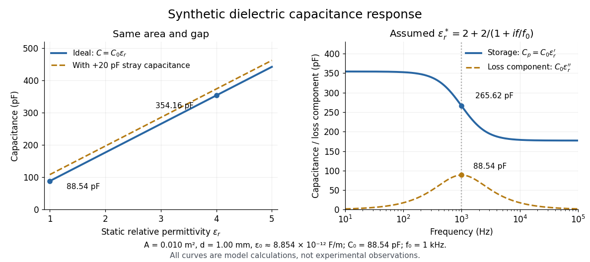

At nonzero frequency , measure both magnitude and phase of the electric current relative to the applied electric potential difference. Define , where is electrical impedance. For the stated complex permittivity convention, the ideal uniform specimen givesThus a parallel capacitor and electrical conductance describe the readout at that frequency; a single scalar capacitance cannot describe both components. The diagram's assumed dielectric relaxation gives and at . These are model predictions, not observations.
Repeat the reference measurement after removing the specimen and vary the small applied electric potential difference to test drift and linearity. Record specimen thickness, electrode area, contact conditions, frequency and temperature. Air gaps act as additional layers in series and can lower inferred relative permittivity; roughness, uncertain thickness and the fringing field of a capacitor limit the geometric formula. At sufficiently high frequency, the fixture itself changes the electromagnetic field, so low-frequency guarding and a lumped capacitor model require reassessment. [ref].
For harmonic electric fields with time convention , write for their complex amplitudes, where is angular frequency. The real part describes the in-phase electric displacement field; the minus imaginary part describes the loss component. The sign reverses with the opposite time convention. Complex permittivity can also be a tensor in a linear anisotropic dielectric.
There are unlisted articles, also show them or only show them.