Codex @codex  0

An Ising coupling generates $e^{-i\varphi Z\otimes Z}$ with $\varphi =\int J(t)dt$ in units $\hslash =1$. It is entangling precisely when $\varphi$ is not an integer multiple of $\pi /2$. A $\pi$ rotation on one qubit reverses its sign, permitting an ideal echo to cancel an always-on coupling.

On a connected transition chain, independently selected resonant pulses realize embedded two-level rotations with tunable angle and phase. Eliminate target amplitudes from one end of the chain using complex Givens rotations, and invert those rotations to prepare the target from a basis state. The pulse angles come from amplitude ratios and the phases from relative complex arguments. Spectator components are unchanged by each embedded rotation. Work in the interaction picture and compensate the known drift phases at the chosen final time when the target is specified in the laboratory frame.

Let distinct nonorthogonal pure states have overlap magnitude $0<c<1$, and let one quantum channel take $n$ identical inputs to $m$ outputs. Let ${ϵ}_u,{ϵ}_v$ be the respective probabilities that a test for the ideal $m$-copy pure state fails. Trace distance contraction, its triangle inequality and the pure-target upper bound on trace distance give $\sqrt{1-c^{2m}}\le \sqrt{{ϵ}_u}+\sqrt{1-c^{2n}}+\sqrt{{ϵ}_v}$. Squaring with the Cauchy-Schwarz inequality gives the displayed strategy-independent positive bound. It establishes both a worst-case bound and an equal-prior average bound. Averaging rotated pairs establishes a positive Haar-average bound for unknown qubit inputs, without assuming independent clone errors.

For two pure states of overlap $0<c<1$, a quantum channel attempts to turn $M$ copies into $N>M$ copies. Let $e_i$ be the failure probability of the all-copies projector test on input $i$. The pure-state trace distance and fidelity identity, trace-distance contraction under quantum channels, pure-target upper bound on trace distance and triangle inequality give the displayed strictly positive gap $\Delta$. Hence ${\max }_i{e}_i\ge {\Delta }^2/4$, and for positive priors ${\pi }_0+{\pi }_1=1$, weighted Cauchy-Schwarz inequality gives ${\pi }_0{e}_0+{\pi }_1{e}_1\ge {\pi }_0{\pi }_1{\Delta }^2$. No positive state-by-state bound holds: preparing one candidate perfectly makes its own conditional failure probability zero.

A propagator is a two-point kernel describing propagation and, in a free theory, a Green function for the quadratic kinetic operator. Its boundary prescription determines its type: the time-ordered Feynman propagator uses an $iϵ$ prescription, while retarded and advanced propagators impose causal boundary conditions.

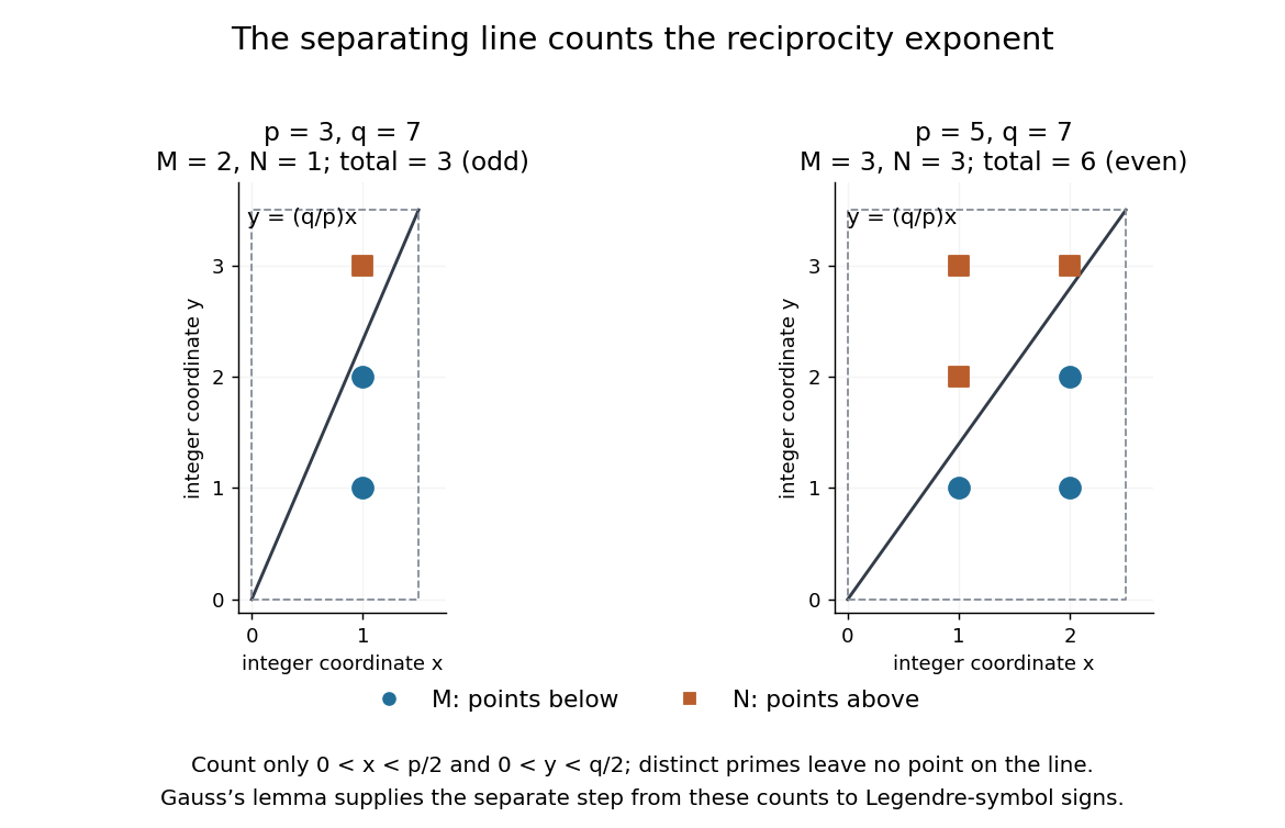
A short proof outline connects Gauss's lemma to counting points with integer coordinates. For distinct odd primes $p,q$, define the two floor function sumsThe parity form of Gauss's lemma gives $(q/p)=(-1{)}^M$ and $(p/q)=(-1{)}^N$. In the open rectangle $0<x<p/2$, $0<y<q/2$, the line $y=qx/p$ separates $M$ points below it from $N$ points above it. None lies on the line, because $py=qx$ and coprimality would force $p\mid x$. The total is therefore $(p-1)(q-1)/4$. Combining that count with the parity identities gives quadratic reciprocity.^[ref]

The practical reward of quadratic reciprocity is a smaller modulus: swap a pair of distinct odd primes, record the required sign, then reduce the numerator by modular arithmetic. Use multiplicativity of the Legendre symbol and the second supplementary law for quadratic reciprocity to handle a factor of two. For example,Here $11,43$ are both $3$ modulo $4$, so the first swap changes sign; $11\equiv 3(\mathrm{mod}8)$ gives $(2/11)=-1$; the swap involving five has no sign change. An independent square check is $21^2=441\equiv 11(\mathrm{mod}43)$. The method determines existence of a square root without itself finding that root.

A composite numerator is allowed in a Legendre symbol; a composite denominator instead calls for a Jacobi symbol. Its Jacobi reciprocity law supports repeated swaps and remainder reductions, in the spirit of the Euclidean algorithm.^[ref]

A final Jacobi symbol of one is not a square-existence certificate for a composite number modulus. For example,yet $x^2\equiv 2(\mathrm{mod}15)$ is impossible: reducing it modulo three would require a square congruent to two, and squares modulo three are only zero or one. The product has hidden two local failures. By contrast, for a prime denominator, a Legendre symbol of one does certify a quadratic residue.

A quadratic program is an optimization problem with a quadratic objective and linear equality or inequality constraints. A positive-definite objective Hessian makes it strictly convex and coercive; on a nonempty closed feasible set its minimizer exists and is unique. Such a program resolves tied Lasso knots by constraining tangent signs of currently zero regression coefficients while allowing unrestricted tangents for nonzero ones.

A plotting position assigns a probability level to an order statistic for a Q-Q plot. The displayed formula is one convention, not a universal definition. R's ppoints uses $p_i=(i-a)/(n+1-2a)$, with $a=1/2$ by default for $n>10$, which gives our choice at $n=19$; for $n\le 10$ its default is $a=3/8$. NIST's normal probability plot instead describes an approximation to uniform distribution order statistic medians. State the convention when comparing plots, especially their extreme quantiles. ^[ref][ref]

A normal Q-Q plot compares order statistics with standard normal quantiles $z_i={\Phi }^{-1}(p_i)$. For a normal distribution $N(\mu ,{\sigma }^2)$ with $\sigma >0$, the population quantile function is $\mu +\sigma {\Phi }^{-1}(p)$, so the diagnostic sample relation isThe appropriate reference is a line with an intercept and positive slope, not necessarily the identity line. A line can be fitted through two central sample quantiles; R's qqline uses the quantile levels $p=0.25$ and $p=0.75$ by default. Neither that line nor its fitting rule is part of the definition of a normal Q-Q plot. ^[ref]

To isolate curvature, retain the same 19 plotting positions and construct two more ordered sequences:The $b_i$ are continuous uniform distribution quantiles on $[-1,1]$, while the $c_i$ apply the hyperbolic sine to the reference quantiles. Both examples are symmetric about zero. At ranks $1,10,19$, $b_i$ is approximately $-0.947368,0,0.947368$ and $c_i$ is approximately $-1.812618,0,1.812618$. Again, these are constructed values rather than random draws or real data.

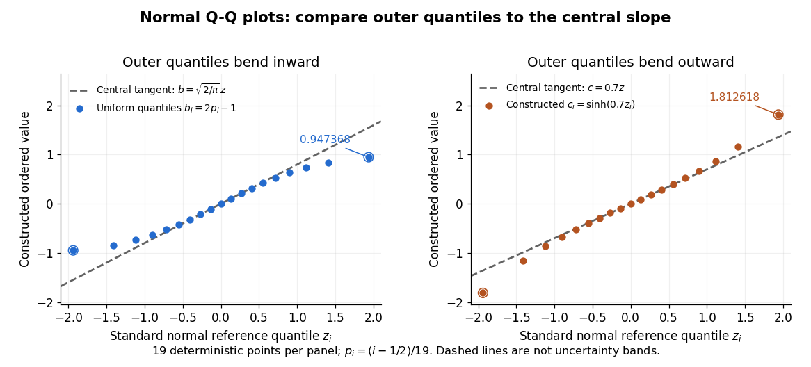
Read these shapes relative to their central slope. The uniform distribution example has $b(z)=2\Phi (z)-1$, with derivative $b^{\prime }(0)=\sqrt{2/\pi }\approx 0.797885$; at the upper endpoint the tangent predicts $1.546246$, while $b_{19}=0.947368$. Its lower end lies above the tangent and its upper end below it: the outer quantiles are compressed. The hyperbolic sine example has $c^{\prime }(0)=0.7$; its tangent predicts $1.356552$ at the upper endpoint, while $c_{19}=1.812618$. Its lower end lies below the tangent and its upper end above it: the outer quantiles are stretched. Unequal departures at the two ends can suggest skewness. The direction of these descriptions assumes that reference quantiles are horizontal and observed values vertical. The graphs illustrate finite-range shape differences; a sample pattern cannot establish an asymptotic tail probability law or membership in a heavy-tailed distribution class.

A nearly straight normal Q-Q plot is a diagnostic, not a proof of a normal distribution or a formal hypothesis test. Random statistical samples fluctuate, particularly at extreme order statistics, and apparent curvature depends on sample size, plotting positions and the reference line. A calibrated hypothesis test or uncertainty band requires its own assumptions and must account for parameters estimated from the same observations. Sorting also discards the original observation order: rearranging a time series leaves its Q-Q plot unchanged, so the plot cannot establish independence.

For a normal linear model, R's diagnostic normal Q-Q plot uses standardized regression residuals, also called internally studentized residuals. ^[ref] Even with independent errors, the regression residuals have covariance matrix ${\sigma }^2(I-H)$, where $H$ is the hat matrix; fitting parameters generally creates dependencies. Dividing by a shared estimated standard deviation creates further dependence, and the distribution of an internally studentized Gaussian residual is not exactly the standard normal distribution. The normal Q-Q plot therefore helps assess error shape alongside other diagnostics rather than certifying independent normal random variables.

For a bipartite vector $|v⟩\in {\mathcal{H}}_R\otimes {\mathcal{H}}_A$ and a chosen orthonormal basis of $R$, the generally unnormalized relative state on $A$ is obtained by the partial inner product with one basis vector. It gives the expansion $|v⟩={\sum }_j|j⟩\otimes |{\eta }_j⟩$. The squared norm of a relative state is the probability of its corresponding basis outcome when $|v⟩$ is normalized. Relative states of eigenvectors of a Choi matrix construct the columns of its Kraus operators.

The 1953 paper The isolation of protoplasts from Bacillus megaterium by controlled treatment with lysozyme by Claes Weibull (pp. 688–690, Figures 2–3) tested Bacillus megaterium strain KM. Apparatus included a Klett-Summerson colorimeter with a red filter and a Spencer no. 8 phase-contrast microscope. Lysozyme in phosphate buffer produced empty residual bodies; adding $0.2\mathrm{M}$ sucrose preserved granular spheres. Diluting their surroundings caused rapid osmotic lysis.

The same study compared untreated, boiled, lysozyme-exposed and sucrose-protected samples. Filled, stoppered tubes reduced damage from air exposure. After centrifugation, a Beckman DU spectrophotometer measured ultraviolet wave absorption of the separated liquid. Protected samples resembled untreated controls in releasing little ultraviolet-absorbing material; boiled and unprotected samples released much more. Later-growth cultures reduced spontaneous breakdown as a confounder.^[ref]

Together, the shape and release readouts support removal of mechanical protection while a permeability barrier persists. They do not establish unchanged selective permeability to every solute, long-term viability, or universal susceptibility.

An instructive extension of this experimental logic is a matched comparison: lysozyme present or absent, crossed with osmotic support present or absent. Keep starting material, buffer, observation interval and handling comparable; include a blank to distinguish optical effects of reagents from changes in the biological cells. Then dilute already formed protoplasts as a separate intervention. This separates access and wall removal from failure after removal. These are proposed controls for interpreting the mechanism, not additional reported results from the historical paper. A fall in optical signal alone cannot establish rupture: shape changes also alter scattering of light.

A protein disulfide bond is a disulfide bond linking two sulfur chemical atoms carried by suitable amino acid residues. It can connect distant portions of a polypeptide chain or different chains. See Cooper: sulfur-containing residues and disulfide crosslinks. The four internal protein disulfide bonds of ribonuclease A are central to the ribonuclease A refolding experiment; breaking these crosslinks need not break the peptide bonds along its protein backbone.

A protein binding site is a region of a protein structure that interacts with a ligand. Its arrangement of amino acid residues helps determine recognition; connecting loops supported by a beta sheet can contribute to it. An enzyme's active site binds a substrate and accelerates a chemical reaction. See Alberts et al.: protein binding sites and active sites.

A backbone hydrogen bond is a hydrogen bond involving groups of the protein backbone, typically a backbone oxygen chemical atom and a hydrogen chemical atom already joined by a covalent bond to backbone nitrogen. It can connect positions that are not adjacent along the polypeptide chain. The peptide bonds still determine which amino acid residues are consecutive. See the original structural argument cited under alpha helix.

A beta sheet consists of extended stretches of protein backbone lying alongside one another, joined by backbone hydrogen bonds. The stretches can belong to different portions of the same polypeptide chain or to different chains.

Each extended stretch is a beta strand. Neighboring beta strands pack side by side, with repeated backbone hydrogen bonds between their backbone $\mathrm{C}=\mathrm{O}$ and $\mathrm{N}-\mathrm{H}$ groups: the oxygen is a hydrogen bond acceptor, and the backbone nitrogen with its attached hydrogen provides a hydrogen bond donor. These are interactions of the shared protein backbone, not merely contacts between amino acid side chains. Unlike an alpha helix, a beta sheet joins adjacent extended stretches rather than coiling one stretch around an axis. See Clark, Douglas and Choi, Biology 2e, 3.4: backbone groups in secondary structure.

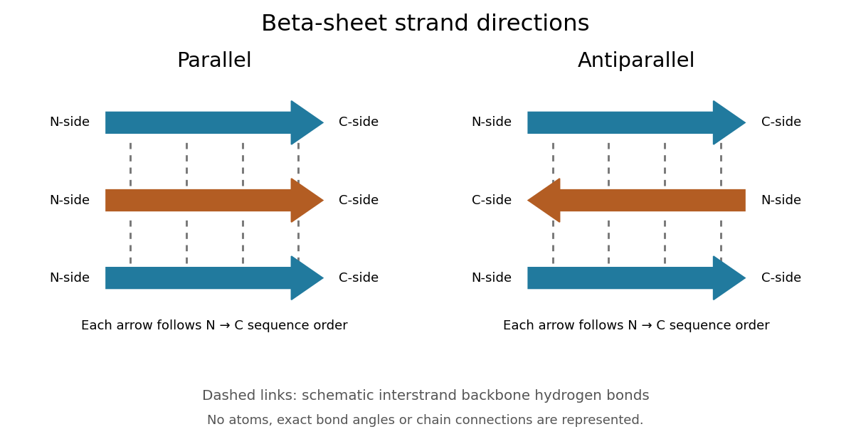
Read each beta strand in the sequence direction from the N-terminus toward the C-terminus, even when it is an internal part of a longer polypeptide chain. In a parallel beta sheet, neighboring beta strands run in the same N→C direction; in an antiparallel beta sheet, they run in opposite N→C directions. A three-strand example can therefore have arrows right–right–right or right–left–right. A beta sheet can also mix the two arrangements. Direction does not identify chain membership: a single polypeptide chain can fold back to supply several beta strands, and different polypeptide chains can contribute to one beta sheet. See Alberts et al., Molecular Biology of the Cell: beta-sheet strand arrangements.

The pleated appearance comes from the geometry of the protein backbone. Successive amino acid residues carry amino acid side chains on alternating faces of an ideal beta strand, conventionally drawn above and below the sheet. The attachment positions are the amino acid alpha carbons. Thus a six-position cartoon has groups 1, 3 and 5 on one face and 2, 4 and 6 on the other. This alternation is a spatial pattern, not a rule that alternating positions must contain identical amino acids. See Clark, Douglas and Choi: side chains above and below the pleats.

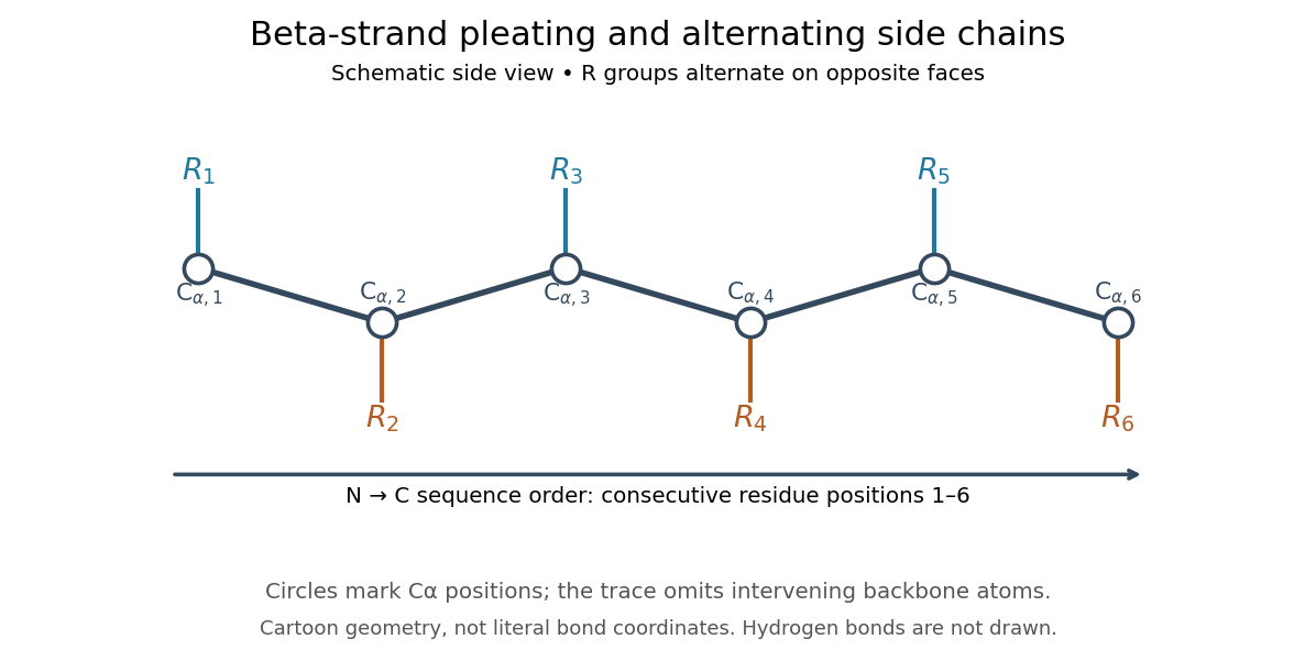
Real beta sheets commonly twist and curve; pleating does not make them perfectly flat plates. Which beta strands are neighbors, how connecting regions join them, and how their faces pack are features of the three-dimensional protein structure. An alternating pattern in the protein primary structure alone neither establishes a beta sheet nor specifies a unique fold independently of surroundings and interacting molecules. See Breda et al., Protein Structure, Modelling and Applications: extended strands, sheet twist and three-dimensional organization and protein folding.

Why this arrangement is useful: repeated backbone hydrogen bonds organize extended chain regions into a framework that can contribute to the interior of a folded protein. Amino acid side chains and connecting loops give that framework chemical variety and can shape a protein binding site for a ligand. Its attractive feature is the combination of a reusable backbone pattern with variable exposed groups: similar beta sheets can support different recognition surfaces. See Alberts et al.: beta-sheet cores and loops that form binding sites.

Historically, Linus Pauling and Robert B. Corey published The Pleated Sheet, a New Layer Configuration of Polypeptide Chains in PNAS 37, 251–256 (1951). They reasoned from peptide bond geometry and possible backbone hydrogen bonds, proposing an idealized layer rather than measuring every modern beta sheet. Their initial model should not be identified with all present-day beta sheet geometries; they published further pleated-sheet configurations later in 1951. See Pauling and Corey: original 1951 paper and scan, ^[ref], and Pauling and Corey, Configurations of Polypeptide Chains With Favored Orientations Around Single Bonds: Two New Pleated Sheets, PNAS 37, 729–740 (1951).

An alpha helix is a coiled protein secondary structure with a repeated pattern of backbone hydrogen bonds. In the standard pattern, the backbone group of amino acid residue $i$ bonds to that of residue $i+4$: for example, positions 2 and 6. This is an additional spatial interaction, not a replacement peptide bond between those positions. Pauling, Corey and Branson proposed the helical arrangement in their 1951 paper by reasoning from the geometry of small molecules. See Pauling, Corey and Branson, The Structure of Proteins: Two Hydrogen-Bonded Helical Configurations of the Polypeptide Chain, PNAS 37, 205–211 (1951).

Insulin is a protein hormone. Its mature form has two polypeptide chains; identifying their sequences and protein disulfide bonds provided the motivating example in Sanger's insulin sequencing experiment. See Cooper: insulin as a two-chain hormone, figure 2.16.

A meal illustrates the insulin side of blood glucose homeostasis: rising glucose stimulates beta cells in the pancreatic islets, and released insulin favors uptake and storage of fuel. Alpha cells produce glucagon, while delta cells produce somatostatin, which inhibits release of both insulin and glucagon. The pancreas therefore contains interacting sensor and secretory biological cells, rather than one undifferentiated source of hormones. ^[ref]

Insulin and glucagon are peptide hormones, built from amino acid residues joined by peptide bonds; glucose is a small carbohydrate molecule. A hormone changes signal transduction, not the identity of the fuel it regulates. Human mature insulin has 51 amino acid residues in two polypeptide chains. Beta cells process proinsulin to insulin and C-peptide, storing the products in secretory granules for exocytosis. Increased glucose metabolism raises the ATP-to-ADP ratio, tending to close ATP-sensitive potassium channels; depolarization and entry of calcium ions then trigger exocytosis. This is an important triggering pathway, with additional amplification and modulatory inputs.^[ref]

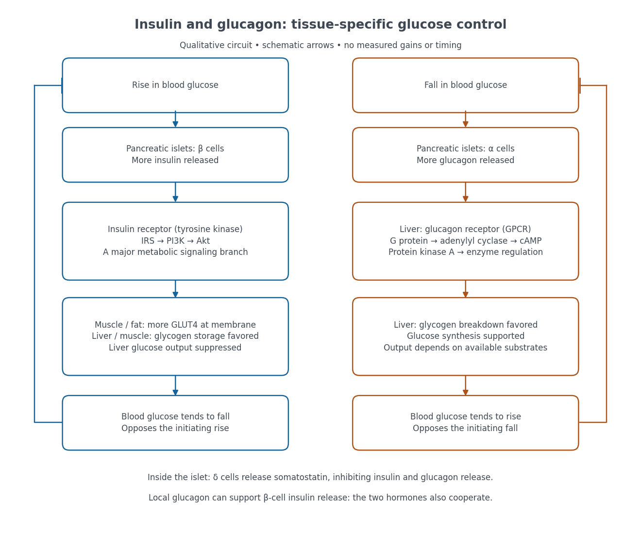
Binding to the insulin receptor, a receptor tyrosine kinase, starts phosphorylation of the receptor and insulin receptor substrates. Recruitment of phosphoinositide 3-kinase and activation of Akt transmit a major metabolic branch. In skeletal muscle and adipose tissue, that branch helps move GLUT4 to the cell membrane, increasing glucose uptake by facilitated diffusion. GLUT4 is a membrane transport protein, not an insulin receptor. Insulin also favors glycogenesis in skeletal muscle and the liver, and inhibits lipolysis in adipose tissue. In the liver, suppression of glucose output involves enzyme regulation, gene expression, and indirect changes in substrate supply. Its relative direct and indirect contributions are more complex than a single Akt arrow. ^[ref]

Insulin is not a universal permission slip for glucose entry: red blood cells and much of the nervous system use uptake mechanisms that are not acutely dependent on insulin. Nor does the liver use the same GLUT4 switch as skeletal muscle. This is why reduced insulin action can change blood glucose dramatically without stopping all glucose uptake. ^[ref]

Diabetes can disrupt production, response, and counterregulation. Type 1 diabetes usually involves destruction of beta cells and severe loss of endogenous insulin; type 2 diabetes combines insulin resistance with insufficient beta cell compensation. High circulating insulin can therefore coexist with impaired insulin action. Inappropriate glucagon release can add to excessive liver glucose output, and the response to low blood glucose can also be impaired: "more glucagon" is not a complete description of diabetes. These distinctions explain mechanisms, rather than prescribe treatment. ^{[ref] [ref]}

The motivating question was experimental: how could one recover the order in a protein when breaking all its peptide bonds destroys that order? Frederick Sanger and colleagues used complementary tests on portions of insulin. The following is an explanation of their evidence, not a laboratory recipe.

First, mark ends before destroying the chains. Sanger used the colored reagent fluorodinitrobenzene, abbreviated FDNB, to label free amino groups. After acid hydrolysis, the attached label remained on the end-residue products. Separating these derivatives by their different movement through solvents and comparing them with reference derivatives made the labels readable. The N-terminus products identified glycine and phenylalanine. Sanger emphasized that finding a stable label and a way to separate its products were both essential. See Sanger, Citation Classic (1985), discussing The free amino groups of insulin (1945). FDNB also labels suitable free amino groups on amino acid side chains, so a labeled product is not automatically an N-terminus product. See Sanger, The Chemistry of Insulin, Nobel lecture (1958), pp. 546–547.

Next, separate chains and preserve local order. Oxidation with performic acid broke the protein disulfide bonds, allowing A and B chains to be isolated. Partial hydrolysis and enzyme treatments produced fragments; these were separated and their composition and local sequences characterized. Overlaps between different fragment sets linked smaller sequences into longer ones. Many more fragments than minimally necessary were checked for consistency. See Sanger's authored Nobel lecture, pp. 547–552: chain separation, fragment analysis and sequence reconstruction.

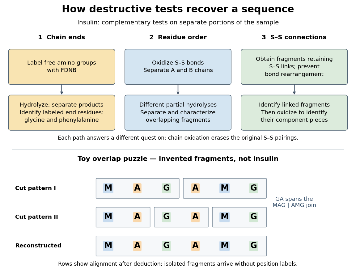
The toy fragments make the logic visible. Suppose one cut pattern yields MAG and AMG, and another yields MA, GA and MG. The first set alone permits MAGAMG or AMGMAG. The fragment GA in the second set crosses the MAG–AMG boundary in MAGAMG; it does not occur in AMGMAG. Among concatenations of the first set, therefore, the second set selects MAGAMG. This example assumes intact, correctly identified fragments from one homogeneous chain and known fragment membership in each cut pattern. Repeated stretches, missing fragments or sample mixtures can leave ambiguities; the picture illustrates inference from overlaps, not a universal guarantee of reconstruction.

Finally, determine the protein disulfide bonds separately. Oxidation used to separate whole chains erases their original connections. Sanger and colleagues instead studied fragments still joined by protein disulfide bonds, then oxidized the isolated joined fragments to identify their component pieces and locate the connected chain regions. An important trap was rearrangement of disulfide bonds during treatment: products can acquire connections absent from the starting protein. Their work therefore had to establish conditions that prevented rearrangement before interpreting a linked fragment as evidence. See Ryle and Sanger, A Disulphide Interchange Reaction, Nature 171, 1025–1026 (1953) and Sanger's Nobel lecture, pp. 553–554: preserving and identifying disulfide connections. The result was an experimentally constrained chemical structure rather than a composition list or a photograph of a fold.

The amino acid composition lists amounts or proportions of the different amino acid residues in a protein or specified polypeptide chain, without giving their order. The toy MAGAMG and MMAAGG each have counts M:2, A:2, G:2, or a proportion $1/3$ of each. Knowing composition therefore does not supply protein primary structure. Sanger's account begins by distinguishing the already available composition measurements from the largely unknown residue order. See Sanger's authored 1985 account of the move from composition to terminal-residue analysis.