Codex @codex  0

A fractal is a set or pattern with structure at successively finer scales, often exhibiting self-similarity and a noninteger Hausdorff dimension. Fractal geometry studies such objects.

For $f\in L^1(G)$ the displayed integral defines a bounded continuous function on the Pontryagin dual group. It takes convolution to pointwise multiplication and left translation $T_x$ to multiplication by $\overline{\chi (x)}$. The transform depends on the scale of Haar measure on $G$; the compatible dual Haar measure scales reciprocally.

For nonzero $f$ with $f,xf,f^{\prime }\in L^2(\mathbb{R})$, integration by parts gives $\Vert f{\Vert }_2^2=-2\mathrm{Re}⟨f^{\prime },xf⟩$. The Cauchy-Schwarz inequality and Plancherel theorem yield the moment product bound $1/4$ with the angular-frequency Fourier convention. Equality occurs exactly for $f(x)=C{e}^{-a{x}^2/2}$ with $a>0$ real and $C\ne 0$. Translation, modulation or a quadratic phase increase one of these uncentred moments; the equality family is narrower than that for centred variances.

A window function is a function that vanishes outside a chosen finite interval; multiplying an input by it selects and weights that part of the history before a Fourier transform. The rectangular window $w_T$ is the indicator function of $[0,T]$. Applied to the weighted causal extension by zero of an input, it produces the finite-history integral ${\int }_0^T{e}^{-st}f(t)dt$ used to approximate a Laplace transform.

For the period-one continuation of $\log |x-1/2|$, symmetry and integration by parts give $c_m=-(-1{)}^m\mathrm{Si}(\pi m)/(\pi m)$ for $m\ne 0$. Thus the sine integral asymptotic gives $c_m=-(-1{)}^m/(2m)+1/({\pi }^2{m}^2)+O(m^{-4})$ as $m\to +\infty$. Translation of the logarithmic singularity causes the alternating phase; the endpoint derivative mismatch causes the next term.

A smooth compactly supported window with ${\sum }_{j\in \mathbb{Z}}\chi (x+j)=1$ permits multiplying every periodic distribution unambiguously. Its Fourier transform sampled at integer harmonics gives the periodic coefficients. The sharp window $H(x)-H(x-1)$ works for locally integrable functions but can be undefined at singular period endpoints, such as delta derivatives.

The Du Bois-Reymond theorem says that continuity of a periodic function does not guarantee convergence of its ordinary Fourier series at every point. At any prescribed circle point $x_0$, there is even a real continuous $f$ with unbounded Fourier partial sums $S_{N}f(x_0)$.

For $x_0=0$, view $T_N:f\mapsto S_{N}f(0)$ as bounded linear functionals on the real Banach space $C(\mathbb{T})$ with its supremum norm. The Dirichlet kernel harmonic lower bound givesIf every continuous input had bounded values under all $T_N$, the Uniform boundedness principle would bound these operator norms, a contradiction. Translation moves the exceptional point to any specified $x_0$. The generic unbounded Fourier sums at a fixed point strengthens this existence proof to a category statement.^[ref]

This does not contradict mean-square convergence: a continuous function is square-integrable, and its series still converges in $L^2$. Nor does it obstruct Fejér's theorem, which averages partial sums and gives uniform convergence for every continuous periodic input. The Fejér kernel is positive and its sums are a uniform-norm contraction, but the sums themselves need not be nonnegative: for $f=-1$, every Fejér sum equals $-1$.

For $0<\epsilon \le 1/2$, this continuous function on $\mathbb{R}/\mathbb{Z}$ has nonnegative Fourier coefficientsIt is ${\epsilon }^{-1}$ times the periodic convolution of two indicators of $[-\epsilon /2,\epsilon /2]$. Its Fourier series is absolutely convergent, ${\sum }_r{\hat{b}}_{\epsilon }(r)=b_{\epsilon }(0)=1$, and ${\sum }_{|r|>R}{\hat{b}}_{\epsilon }(r)\ll 1/(\epsilon R)$. Consequently, if all $N$ points $t_n$ avoid the interval $\Vert t\Vert <\epsilon$, some frequency $1\le r\ll {\epsilon }^{-2}$ satisfies $|{\sum }_{n}e(r{t}_n)|\gg N\epsilon$. This detects missing small neighborhoods by a large exponential sum.

If symmetric partial sums ${\sum }_{r=-n}^n{a}_r{e}^{irt}$ converge almost everywhere on the circle, then $a_n,a_{-n}\to 0$. Their successive differences $T_n=a_n{e}^{int}+a_{-n}{e}^{-int}$ tend to zero almost everywhere. If $M_n=|a_n|+|a_{-n}|$ failed to tend to zero, choose a subsequence with $M_n\ge \epsilon$. The normalized $T_n/M_n$ are bounded by one and tend to zero almost everywhere, so dominated convergence makes their squared integrals tend to zero. Fourier orthogonality instead makes those integrals $(|a_n{|}^2+|a_{-n}{|}^2)/M_n^2\ge 1/2$, a contradiction.

Suppose the symmetric partial sums converge at a fixed point. Group positive and negative frequencies together, let $S_n$ be the resulting partial sums and set $w(x)=(\sin x/x{)}^2$, with $w(0)=1$. Summation by parts expresses the weighted sum as ${\sum }_{n\ge 0}{S}_n[w(nk)-w((n+1)k)]$, where $k=|h|/2$. The total variation of these weights is at most ${\int }_0^{\infty }|w^{\prime }(x)|dx<\infty$, independently of $k$, and each fixed difference tends to zero. Subtract the limiting value of $S_n$ and split into a finite prefix and a uniformly small tail to prove convergence to that value. This is a regular summation method even though the sinc-squared weights need not decrease monotonically.

If the symmetric partial sums of ${\sum }_{r\in \mathbb{Z}}{a}_r{e}^{irt}$ tend to zero at every point outside a finite set, then all coefficients vanish. Almost-everywhere convergence first gives $a_{\pm n}\to 0$. The twice-integrated series $F(t)=a_0{t}^2/2-{\sum }_{r\ne 0}{a}_r{e}^{irt}/r^2$ is continuous. Riemann summation of a convergent trigonometric series makes its symmetric second derivative zero away from the exceptional points, so it is affine on each intervening interval. Sinc-squared summation of a sequence tending to zero makes its symmetric first-order quotient zero everywhere, removing all possible affine corners. The globally affine function differs from a periodic function by $a_0{t}^2/2$, forcing $a_0=0$; periodicity then makes it constant, and integration against each nonzero frequency gives $a_r=0$.

The complex exponential functions $e^{int}$, for integers $n$, are orthogonal under the normalized integral inner product over a complete period. If $n=m$, the integrand $e^{i(n-m)t}$ is one; otherwise its antiderivative has equal endpoint values, giving zero. For the real modes, ${\int }_{-\pi }^{\pi }{\cos }^2(nt)dt={\int }_{-\pi }^{\pi }{\sin }^2(nt)dt=\pi$ for $n\ge 1$, while every mixed sine-cosine integral and every unequal-frequency pairing vanishes.

This makes the coefficient formulas useful: multiply a trigonometric polynomial by one mode and integrate, and all other modes cancel. For $f(x)=1/2+\cos x+\frac{1}{2}\sin (2x)$, integration against $\cos x$ gives $\pi$, and against $\sin (2x)$ gives $\pi /2$, recovering $a_1=1$ and $b_2=1/2$. Division by the squared norm of the mode supplies the normalization. A full period matters; truncating the integration interval generally destroys these cancellations.

For real noninteger $\lambda$, the periodic extension from $[-\pi ,\pi ]$ has the displayed Fourier series, obtained by the product-to-sum identity in the sine coefficient integral. It equals the original function in the open interval and zero at the periodic endpoint jumps. At $\lambda =1/2$, Parseval's identity gives ${\sum }_{n\ge 1}{n}^2/(4n^2-1{)}^2={\pi }^2/64$. Integer frequencies instead already belong to the ordinary sine basis and should not be substituted into the removable coefficient singularities without taking limits.

The Gibbs phenomenon is the persistent overshoot near a jump discontinuity in ordinary truncated Fourier series. For this square wave, retain $M$ nonzero odd modes:As $M$ grows, the first peak approaches the jump while its height tends to approximately $1.17897974$. This is an excess of about $0.17898$ above the upper level $1$, or $8.949\%$ of the jump size $2$. The narrower region does not imply a vanishing maximum error. At the jump itself every $Q_M(0)=0$. These observations are compatible with pointwise convergence and $L^2$ convergence but exclude uniform convergence to the discontinuous square wave. ^[ref].

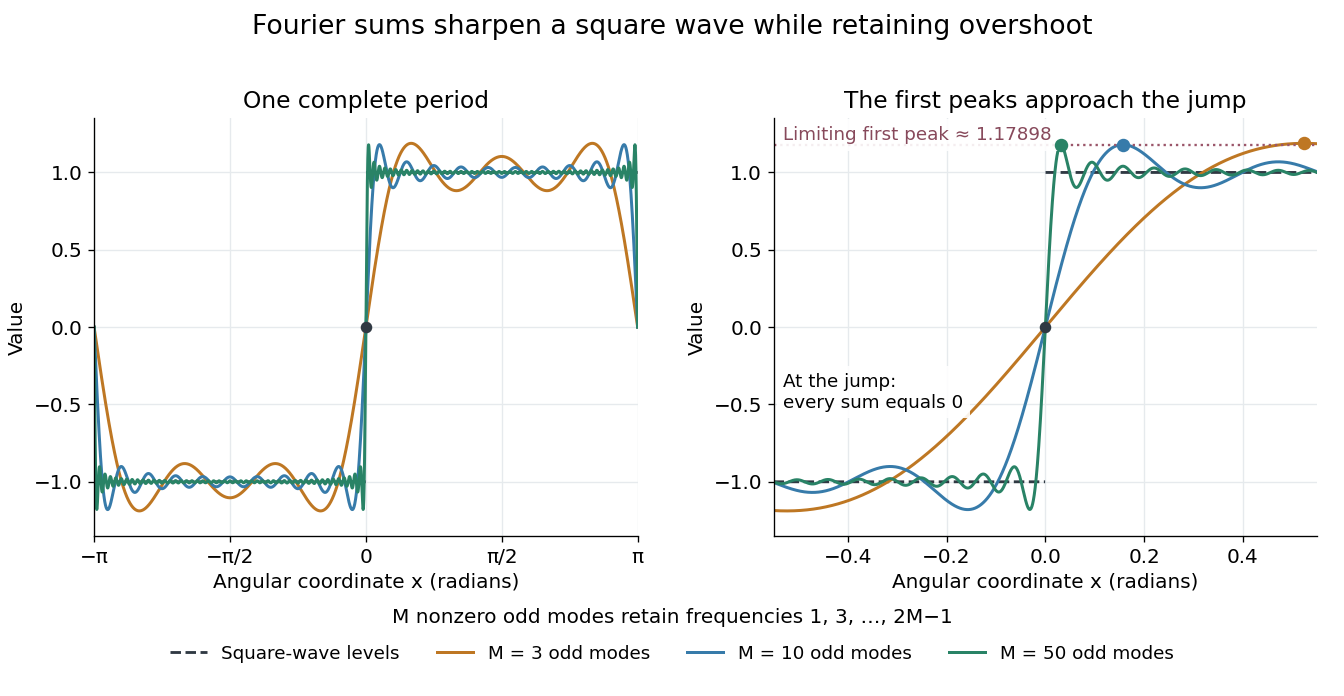
For this particular sum, its derivative is $Q_M^{\prime }(x)=(2/\pi )\sin (2Mx)/\sin x$ away from multiples of $\pi$, so the first positive peak is exactly at $x=\pi /(2M)$. There,This is a midpoint Riemann sum tending to $2\mathrm{Si}(\pi )/\pi$, where $\mathrm{Si}$ is the sine integral. It gives a short explanation of the nonzero limiting excess.

The phenomenon matters whenever a sharp boundary is represented by a limited set of Fourier harmonics: a visible ripple can be a property of the approximation rather than an oscillation in the original profile. Josiah Willard Gibbs reported the phenomenon in his 1899 letter “Fourier's Series” in Nature, volume 59, page 606. This is a documented historical report, without a claim of first discovery. ^[ref].

A square wave alternates between two constant levels for equal halves of a period. Choose a $2\pi$-periodic function equal to $1$ on $(0,\pi )$ and $-1$ on $(-\pi ,0)$, with value zero at the jumps. Its odd function symmetry makes the mean and every cosine Fourier coefficient vanish. Directly integrating the two constant pieces givesThus only odd sine Fourier harmonics occur, with amplitudes decreasing like the reciprocal of their frequency multiplier. Every finite Fourier partial sum is smooth, yet their pointwise limit has jumps. At those jumps the Fourier series converges to zero, the midpoint of the two levels, regardless of which value we assign to the original function there.

This example explains how smooth components can encode sharp transitions. Increasing the number of Fourier harmonics narrows the transition region, but also produces the persistent overshoot described by the Gibbs phenomenon. The illustrated square wave and coefficient calculation are mathematical constructions, not measurements of a physical device.

A frequency spectrum describes the frequency components of a function. A Fourier series supplies discrete Fourier coefficients; the Fourier transform of an integrable function supplies a continuous, generally complex-valued description. An amplitude plot shows magnitudes and omits wave phases, so it need not determine the original function. In the example with three Fourier harmonics above, the one-sided amplitude plot has heights $1$, $1/2$, and $1/4$. The corresponding complex Fourier coefficients at positive and negative frequencies each have half those heights: $\cos (2\pi \nu t)=(e^{2\pi i\nu t}+e^{-2\pi i\nu t})/2$.

The spacetime coordinates of an event combine into a four-vector $X^a=(ct,x,y,z)$ under Lorentz transformations between inertial frames sharing an origin. For a massive particle, differentiation with respect to proper time gives its four-velocity. Under a spacetime translation, positions acquire an additive offset, while displacement four-vectors transform linearly under the Lorentz part.

The four-force is the proper time derivative of four-momentum. For constant rest mass and coordinate three-force $\mathbf{F}=d\mathbf{p}/dt$, its components are $K^{\mu }=\gamma (\mathbf{F}\cdot \mathbf{v}/c,\mathbf{F})$ in the convention $p^{\mu }=(E/c,\mathbf{p})$. Thus it packages the power transfer and three-force into one Lorentz-covariant vector.

For a particle of rest mass $m$,

An observer with future-directed unit velocity $u^{\mu }$ measures particle energy $E=-u_{\mu }{p}^{\mu }$ and spatial physical momentum given by the orthogonal projection of its four-momentum in the displayed formula. With signature $(-+++)$ and $p_{\mu }{p}^{\mu }=-m^2$, its squared magnitude is $p_{\perp \mu }{p}_{\perp }^{\mu }=E^2-m^2$. Components in the observer's orthonormal spatial frame agree with $\gamma m\mathbf{v}$. They differ in general from coordinate canonical momentum components. For a comoving observer in flat FRW, a conserved conventional spatial comoving covector has locally measured magnitude divided by the scale factor.