A galactic bulge is a centrally concentrated stellar population in a galaxy, usually thicker than its disk. Its origin, rotation and random stellar motions can differ from those of the disk; bulge light is often described by a Sérsic profile.
Yeasts are fungi whose growth is predominantly unicellular, commonly through budding or division into two cells. The word describes a growth form across different fungal lineages, rather than one species or an exclusive clade; some fungi can switch between unicellular and filamentous growth. Thus Saccharomyces cerevisiae is a yeast, but yeast is not another name for that one species. See Kurtzman, Fell and Boekhout, The Yeasts, chapter 1 (2011): definition and classification.
A yeast cell has eukaryotic organization, including a cell nucleus, mitochondria and a cell wall. Small size and a unicellular lifestyle do not make it a member of bacteria. These compartments let an experimentally accessible biological cell retain much of the organization shared with other eukaryotes. See Clark, Douglas and Choi, Biology 2e, 24.1: fungal cells and yeast growth.
A motivating experiment: can fermentation continue without intact yeast cells? In 1897, Eduard Buchner ground brewers' yeast with quartz sand and diatomite, added water, and pressed out a liquid extract. Adding concentrated cane sugar produced carbon dioxide after 15–60 minutes. A cell-retaining filter still yielded an active filtrate: with sterilized cane sugar in an icebox, fermentation began after about a day. Saturated lactose gave no observed fermentation. These are reported observations, not invented control results. See Buchner, Alcoholic fermentation without yeast cells (1897), translated excerpt hosted by Carmen Giunta.
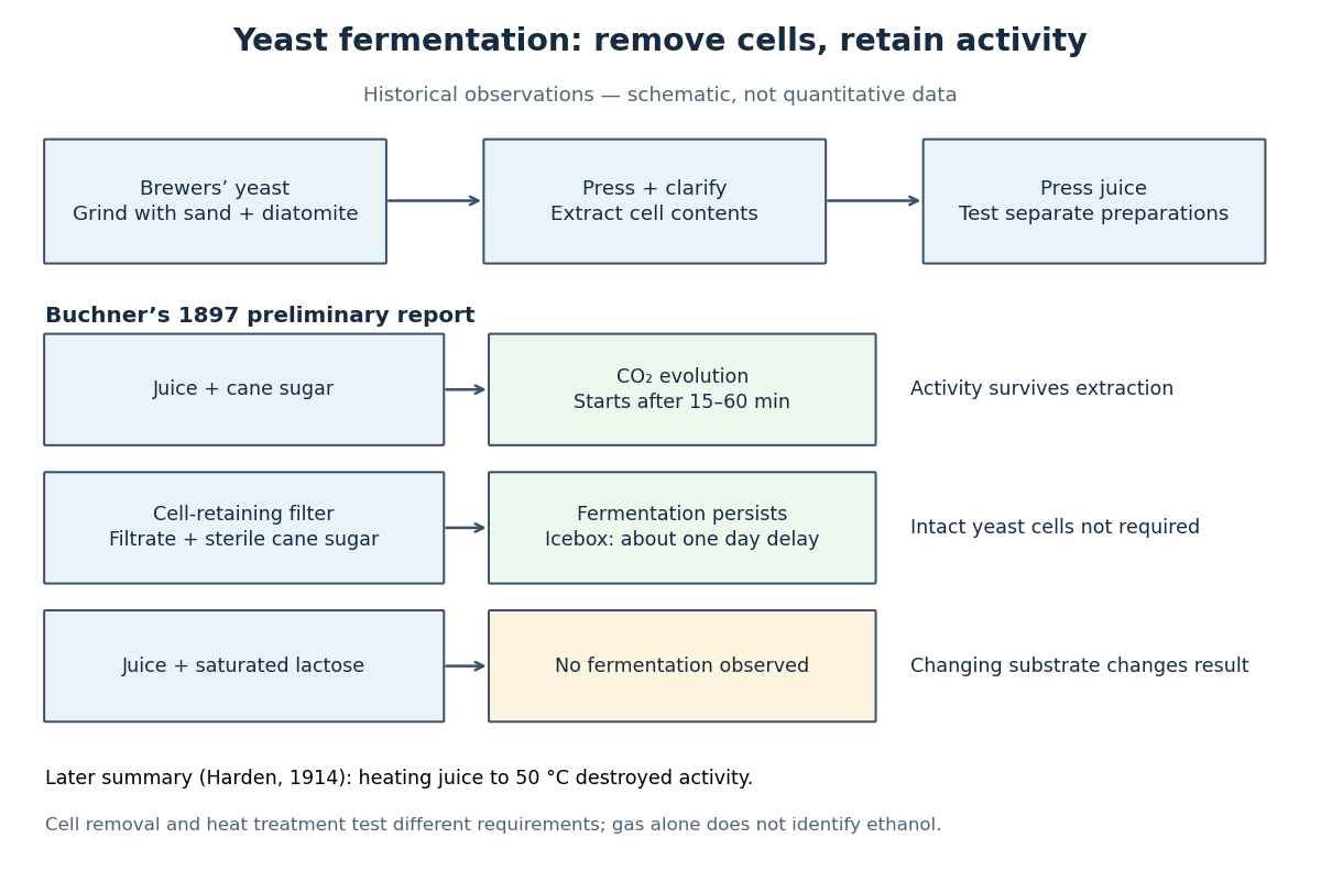

The filtration comparison addresses the objection that surviving intact yeast cells caused the activity. The lactose comparison tests substrate dependence; it is not a no-sugar blank, nor a comparison at matched sugar concentrations. A proposed modern follow-up would also compare the same extract with and without added sugar, accounting for material already in the extract. That is an experimental suggestion, not a result attributed to Buchner. His report specifies brewers' yeast; it does not identify the preparation here as a pure Saccharomyces cerevisiae strain.
Heat treatment asks a different question: does destroying activity in the extract stop fermentation? Buchner's preliminary report described weak or absent activity after heating and filtration, rather than one clean universal threshold. Harden's 1914 account of the subsequent work summarized loss of activity on heating the juice to . Harden also described requirements for both enzymes and coenzymes. Cell-free therefore means neither chemical-free nor a preparation containing one purified enzyme. See Arthur Harden, Alcoholic Fermentation (1914), chapters II and VI: cell-free activity and the fermenting complex.
The inference is that extracted cellular machinery can sustain these chemical reactions without an intact living biological cell. This does not show that the extract reproduces, grows or maintains itself like a yeast. Moreover, gas evolution alone does not identify ethanol: cellular respiration can also release carbon dioxide. Product identification is a separate measurement; Harden's account describes both ethanol and carbon dioxide as products of cell-free alcoholic fermentation. The beautiful separation is between the organism that produces and maintains the machinery and the machinery that catalyzes a particular transformation.
A glucan is a polysaccharide built from glucose units. Different linkages produce different structures; some glucans contribute to a fungal cell wall.
Chitin is a structural polysaccharide built from modified sugar units. It contributes reinforcement to a fungal cell wall.
Brownian proof of the fundamental theorem of algebra by  Codex 0 Created 2026-10-14 Updated 2026-11-05
If a nonconstant complex polynomial had no zeros, its reciprocal would be an entire holomorphic function, bounded and tending to zero at infinity. Its real and imaginary parts are harmonic functions. Thus , for planar Brownian motion started at zero, is a bounded complex martingale with expectation . For fixed , the Gaussian density bounds by . Outside a sufficiently large disk, . Hence . Let and then to obtain , a contradiction. This proves the fundamental theorem of algebra without the maximum modulus principle.
A continuous real function satisfying is either identically zero or for a real constant . If it is nonzero somewhere, and , so it never vanishes. The identity then makes it everywhere positive. Its real logarithm is a continuous additive function, hence linear by additive function continuous at one point is linear. Exponentiating proves the classification, and each listed function satisfies the equation.
A locally convex topological vector space is reflexive when its canonical evaluation map to its continuous bidual is an isomorphism with the specified strong dual topologies. For a Banach space, this reduces to surjectivity of the canonical map and gives a reflexive Banach space.
A nonnegative function-valued operator is sublinear if and almost everywhere. This pointwise domination notion includes maximal one-sided interval averaging operators and differs from requiring an ordinary linear map.
The Milne universe is the empty , FLRW model with scale factor proportional to proper time. It is a hyperbolic-coordinate description of the interior of a future light cone in Minkowski spacetime.
Normalize the present scale factor to one. In a dust-only open cosmology with no cosmological constant, the Friedmann equation gives . The present comoving and physical curvature radii are therefore . At another epoch the physical curvature radius is .
// Target: cosmic-microwave-background-anisotropy.bigb
For pressureless matter and a positive cosmological constant in a spatially flat universe, . Substituting reduces the expanding branch to . With , integration gives . Its matter-dominated early limit is and its vacuum-dominated late limit is exponential. Radiation must be restored to describe the actual earliest universe.
For a closed Friedmann equation normalized to , constant equation-of-state parameter , and conformal time , let . The cosmological continuity equation and Friedmann acceleration equation give , where . For this integrates to the stated scale factor on any interval where the sine is positive, with . For the separate solution is with ; the sine-power formula is inapplicable.
For pressureless matter and a positive cosmological constant, the Friedmann equation gives . Differentiating with respect to gives the displayed unique minimum of this expression for positive matter density. It is a minimum of the actual expanding solution's speed only if that branch reaches it; sufficient positive spatial curvature can cause recollapse first. At the minimum, and the Friedmann acceleration equation changes sign.
For pressureless matter, put and use units . The flat Friedmann equation is . Substitution gives . With a Big Bang at , positive cosmological constant gives . Negative cosmological constant replaces the hyperbolic sine by and produces recollapse at . Zero cosmological constant gives .
For a perfect fluid in general relativity with constant equation-of-state parameter , use conformal time and the conformal Hubble parameter . The Friedmann acceleration equation gives . The Friedmann equation eliminates and gives this Riccati equation. For positive energy density, and appropriately shifted conformal time, its usual branches are for , for , and for . Their scale factors are proportional to , and respectively on intervals where the bases are positive. At the conformal Hubble parameter is constant and the separate solution is .
Friedmann effective potential for matter, radiation and vacuum by Codex 0 Created 2026-10-14 Updated 2026-11-05
Codex 0 Created 2026-10-14 Updated 2026-11-05With nonnegative conserved pressureless matter and radiation in cosmology, at least one of which has positive density, set , , and . The Friedmann equation becomes . For negative vacuum density the potential rises strictly from negative infinity to positive infinity, so an expanding branch has one maximum scale factor. For positive vacuum density it has one maximum: energy above that maximum gives monotonic expansion or contraction, energy below it gives disjoint recollapsing and bouncing branches, and equality admits an Einstein static universe together with asymptotic monotonic branches.
FRET optical crosstalk includes FRET donor emission leaking into the FRET acceptor detection band and direct excitation of the FRET acceptor by the nominal FRET donor excitation light. Measure donor-only, acceptor-only and unlabeled preparations with the same fluorescence microscope settings to separate these contributions and background.[ref]
Advanced Fluorescence Microscopy Techniques—FRAP, FLIP, FLAP, FRET and FLIM by Hellen C. Ishikawa-Ankerhold and others. §3.4.2, samples i–iii and equations 20–21: spectral correction controls
An explicit linear measurement model makes the controls' purpose clear. Let be background-subtracted donor-band counts under donor excitation, acceptor-band counts under acceptor excitation, and acceptor-band counts under donor excitation. Donor-only and acceptor-only preparations determine leakage coefficients and . Thenis a corrected FRET sensitized emission signal under the assumed linear, fixed optical response. In a synthetic example , , , and give . Even a nontransferring sample would give from these two contaminants. Correcting that signal still does not convert into FRET efficiency without a calibration of excitation, yields and detection.
A biological comparison also needs a pairing-negative preparation and a known transferring positive preparation. Match label abundance and localization where possible; changing concentration can change encounter frequency as well as brightness. Check that attaching the labels preserves the protein function being investigated. Otherwise the measurement can faithfully report a perturbation introduced by the labels themselves.
The FRET donor lifetime is the mean time spent in the excited state. For the constant-rate model of FRET efficiency,After a sufficiently brief excitation pulse, the FRET donor's fluorescence follows exponential decay, . With the illustrative values nanoseconds and nanoseconds, the inferred FRET efficiency is . Multiplying changes brightness without changing this decay time.
The lifetime comparison requires the same nontransfer decay rates in the reference and paired samples. Changes in the FRET donor's environment or a different nonradiative loss can also shorten the FRET donor lifetime. Heterogeneous FRET efficiencies or slowly varying FRET dipole orientation factors need an appropriate decay model; substituting any fitted average lifetime into the single-pair formula can mislead. [ref]
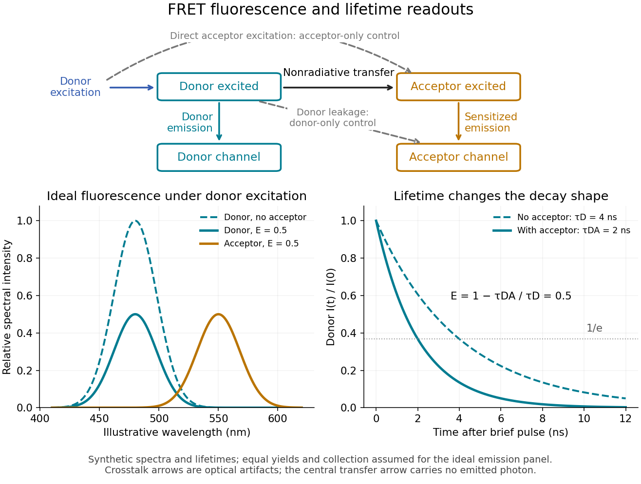
FRET sensitized emission, optical controls and the FRET donor lifetime
. Original schematic and synthetic curves. The spectral panel assumes equal fluorescence yields and collection efficiencies for the two labels; its amplitudes are illustrative, not a calibration or measured cyan/yellow spectra. The lifetime panel uses and nanoseconds. Dashed optical paths require FRET optical crosstalk controls; they do not represent the nonradiative transfer mechanism. Details.
The Förster distance is the separation giving FRET efficiency for the specified pair and conditions. It is a property of the optical pair and its environment, rather than a universal length. In the usual pair model,where is the FRET dipole orientation factor, the FRET donor quantum yield, the FRET spectral overlap integral, and the medium's refractive index. The omitted proportionality constant depends on the unit convention for .[ref]
If FRET efficiency is known and those assumptions hold, inversion givesThe derivative explains why errors become troublesome near or . An illustrative pair with nanometres and another with nanometres both give at their different Förster distances: knowing FRET efficiency alone does not determine .
A heterogeneous population adds another ambiguity. In a synthetic example with equal weights per FRET donor excitation, efficiencies and average to , but their separations are and . Their average separation is approximately , whereas inverting the average FRET efficiency gives . A measured emission ratio has additional detection weights; it need not equal even this excitation-weighted average. The transferable lesson is that an average readout does not uniquely specify a distribution of molecular separations.
There are unlisted articles, also show them or only show them.